可能是史上最详细-Faster RCNN Pytorch 复现全纪录

Faster RCNN复现

文章之前，我们先来明确检测类任务都在干些什么：

需求：

对图像中的特定种类目标做出分类，并求出目标在图像中所处的位置即最终需要的信息：

• object-classes_name
• object-position

在一般的检测任务中类别信息通常由索引代替，例如1-> apple，2 - > cat，3 - > dog，… > 而位置一般可以由两组坐标代替：> 矩形的左上角，右下角坐标（x1，y1，x2，y2）

Faster R-CNN作为两阶段检测网络发展中最重要的一个网络，基本可以视为检测任务的里程碑性成果。

延伸扩展的MaskRCNN，CascadeRCNN都成为了2019年这个时间点上除了各家AI大厂私有网络范围外，支撑很多业务得以开展的基础。所以，Pytorch为基础来从头复现FasterRCNN网络是非常有必要的，其中包含了太多的招数和理论中不会包括的先验知识。

甚至，以Faster RCNN为基础去复现其他的检测网络 所需要的精力和时间都会大大降低

我们的目标：用最简洁，最贴合原文得写法复现Resnet - Faster R-CNN

注：> > 本文中的代码为结构性示例的代码片段，不能够复制粘贴直接运行

架构

VGG16-19因为参数的急剧膨胀和深层结构搭建导致参数量暴涨，网络在反向传播过程中要不断地传播梯度，而当网络层数加深时，梯度在逐层传播过程中会逐渐衰减，导致无法对前面网络层的权重进行有效的调整。

因此vgg19就出现了它的局限性。

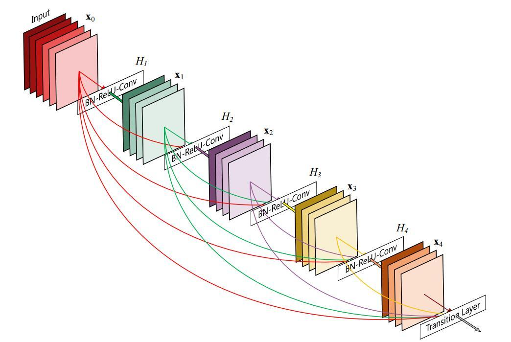
而在之后提出的残差网络中，加入了短连接为梯度带来了一个直接向前面层的传播通道，缓解了梯度的减小问题，同时，将整个网络的深度加到了100层+，甚至后来的DenseNet出现了实用的200层+网络。并且大量使用了1 * 1卷积来降低参数量因此本文将尝试ResNet 101 +FasterRCNN，以及衔接DenseNet和FasterRCNN的可能性。

从以上图中我们可以看出Faster R-CNN除了作为特征提取部分的主干网络，剩下的最关键的也就是以下部分

• RPN`
• RPN LossFunction
• ROI Pooling
• Faster-R-CNN Loss Function

也就是说我们的复现工作要着重从这些部分开始。现在看到的最优秀的复现版本应该是Jianwei Yang page

本文的代码较多的综合了多种写法，以及pytorch标准结构的写法

0.整体流程

先来看看代码（只是大概的看一下就行）：

#################################非Resnet版本只看看基本结构就可以
class FasterRCNN(nn.Module):
    n_classes = 21
    classes = np.asarray(['__background__',
                       'aeroplane', 'bicycle', 'bird', 'boat',
                       'bottle', 'bus', 'car', 'cat', 'chair',
                       'cow', 'diningtable', 'dog', 'horse',
                       'motorbike', 'person', 'pottedplant',
                       'sheep', 'sofa', 'train', 'tvmonitor'])
    PIXEL_MEANS = np.array([[[102.9801, 115.9465, 122.7717]]])
    SCALES = (600,)
    MAX_SIZE = 1000

    def __init__(self, classes=None, debug=False):
        super(FasterRCNN, self).__init__()

        if classes is not None:
            self.classes = classes
            self.n_classes = len(classes)

        self.rpn = RPN()
        self.roi_pool = RoIPool(7, 7, 1.0/16)
        self.fc6 = FC(512 * 7 * 7, 4096)
        self.fc7 = FC(4096, 4096)
        self.score_fc = FC(4096, self.n_classes, relu=False)
        self.bbox_fc = FC(4096, self.n_classes * 4, relu=False)

        # loss
        self.cross_entropy = None
        self.loss_box = None



    @property
    def loss(self):
        return self.cross_entropy + self.loss_box * 10

    def forward(self, im_data, im_info, gt_boxes=None, gt_ishard=None, dontcare_areas=None):
        features, rois = self.rpn(im_data, im_info, gt_boxes, gt_ishard, dontcare_areas)

        if self.training:
            roi_data = self.proposal_target_layer(rois, gt_boxes, gt_ishard, dontcare_areas, self.n_classes)
            rois = roi_data[0]

        # roi pool
        pooled_features = self.roi_pool(features, rois)
        x = pooled_features.view(pooled_features.size()[0], -1)
        x = self.fc6(x)
        x = F.dropout(x, training=self.training)
        x = self.fc7(x)
        x = F.dropout(x, training=self.training)

        cls_score = self.score_fc(x)
        cls_prob = F.softmax(cls_score)
        bbox_pred = self.bbox_fc(x)

        if self.training:
            self.cross_entropy, self.loss_box = self.build_loss(cls_score, bbox_pred, roi_data)

        return cls_prob, bbox_pred, rois

这段代码并不是完整定义，只显示了主要流程，辅助性，功能性的方法全部被省略。
结构也被大大简化
当我们以数据为线索则会产生以下的流程

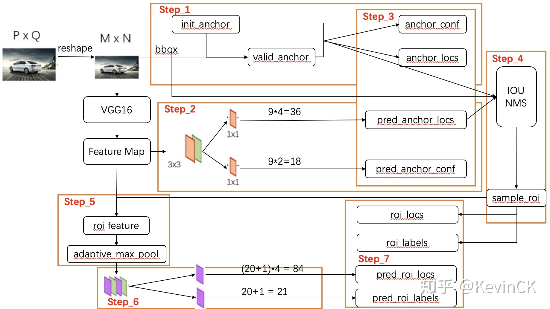
我们在主干网络中可以清晰地看到，向前按照什么样的顺序执行了整个流程（just take a look）

值得注意的是，在以上执行流程中，有些过程需要相应的辅助函数来进行
比如loss的构建，框生成等等，都需要完备的函数库来辅助进行。

以上流程图 ，以及本文的叙述顺序与线索，都是以数据为依托的，明确各个部分数据之间的计算
输入输出信息是非常重要的

初始训练数据包含了：

1.DataLoader

数据加载部分十分自然地,要输入我们的数据集,我们这篇文章使用按最常用的

coco2014/17标准

pascal VOC标准

自定义数据集标准

全部部分当然不能展现 但是我们会在开源项目中 演示Voclike数据集，以及自定义数据集如何方便的被加载->开源-快速训练工具(未完成)

在本文中为了关注主旨我们只介绍自定义数据集和VocLike数据集的加载过程

Data2Dataset

数据的原始形式,当然是以图片为主
我们以一张图为例.

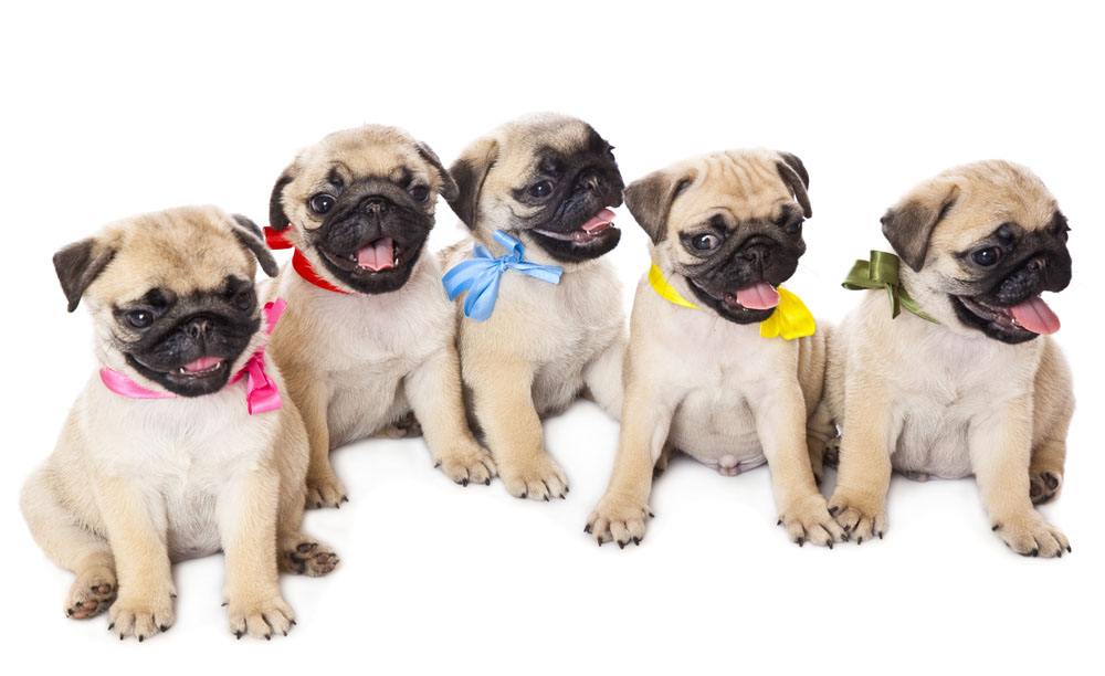
使用labelme标注之后

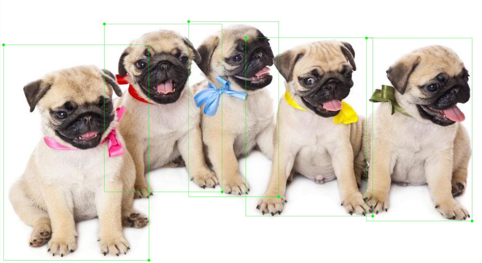
保存之后软件就会自动生成例如：

{
    "version": "3.4.1",
    "flags": {},
    "shapes": [
        {
            "label": "dog",
            "line_color": null,
            "fill_color": null,
            "points": [
                [
                    7,
                    144
                ],
                [
                    307,
                    588
                ]
            ],
            "shape_type": "rectangle"
        },
        ......
        {
            "label": "dog",
            "line_color": null,
            "fill_color": null,
            "points": [
                [
                    756,
                    130
                ],
                [
                    974,
                    507
                ]
            ],
            "shape_type": "rectangle"
        }
    ],
    "lineColor": [
        0,
        255,
        0,
        128
    ],
    "fillColor": [
        255,
        0,
        0,
        128
    ],
    "imagePath": "timg.jpeg",
    "imageData": "此处为base64编码过得图像数据"
}

还有labelimg xml标准的数据样本

<annotation>
	<folder>图片</folder>
	<filename>timg.jpeg</filename>
	<path>/home/winshare/图片/timg.jpeg</path>
	<source>
		<database>Unknown</database>
	</source>
	<size>
		<width>1000</width>
		<height>612</height>
		<depth>3</depth>
	</size>
	<segmented>0</segmented>
	<object>
		<name>dog</name>
		<pose>Unspecified</pose>
		<truncated>0</truncated>
		<difficult>0</difficult>
		<bndbox>
			<xmin>9</xmin>
			<ymin>163</ymin>
			<xmax>309</xmax>
			<ymax>584</ymax>
		</bndbox>
	</object>
....
	<object>
		<name>dog</name>
		<pose>Unspecified</pose>
		<truncated>0</truncated>
		<difficult>0</difficult>
		<bndbox>
			<xmin>748</xmin>
			<ymin>142</ymin>
			<xmax>977</xmax>
			<ymax>508</ymax>
		</bndbox>
	</object>
</annotation>

以及yolo标准的bbox

class_id box
0 0.159000 0.610294 0.300000 0.687908
0 0.346000 0.433824 0.216000 0.638889
0 0.491500 0.449346 0.191000 0.588235
0 0.650000 0.511438 0.246000 0.614379
0 0.863000 0.535948 0.230000 0.588235

yolo的box值最终会由下面的方法转换为标准的框数据(xywh)

def convert(size, box):  # 归一化操作
    #size图像尺寸
    #box包围盒
    dw = 1. / size[0]
    dh = 1. / size[1]
    x = (box[0] + box[1]) / 2.0
    y = (box[2] + box[3]) / 2.0
    w = box[1] - box[0]
    h = box[3] - box[2]
    x = x * dw
    w = w * dw
    y = y * dh
    h = h * dh
    return (x, y, w, h)

Dataset2Dataloader

很多对Faster RCNN复现的版本中，标准的数据加载流程没有被固定化，所以数据被以各种datalayer ，roidb等等方法包装，Pytorch0.4之后，实质上已经出现了最标准化的数据输入形式
即：

一般情况下数据从原始形式，也就是上一节获取到的图片以及label的类别坐标信息。
我们假设以字典单位来承载这个数据单元

因此我们设getdata()为从一个数据列表的json对象中返回我们需要的指定信息

• image
• bboxlist
• classlist
• scale

这其中bboxlist指的是一张图像中所有目标标注框构成的列表，classlist指的是类名，并保证两个列表索引对齐

有了这些设计目标，我们就可以开始构建代码了

class Dataset:
    def __init__(self, opt):
        self.opt = opt
        self.db = VOCBboxDataset(opt.voc_data_dir)
        #定义原始数据的来源如果是自定义数据可以尝试设置数据的列表，然后利用一个通用的读取器来读取数据
        self.tsf = Transform(opt.min_size, opt.max_size)

    def __getitem__(self, idx):
        image, bboxlist, classlist= self.db.get_example(idx)
        img, bbox, label, scale = self.tsf((image, bboxlist, classlist))#对原始数据的变换操作
        # TODO: check whose stride is negative to fix this instead copy all
        # some of the strides of a given numpy array are negative.
        return img.copy(), bbox.copy(), label.copy(), scale

    def __len__(self):
        return len(self.db)

其中变换操作，是为了使得数据转换为张量，以及对数据的平移旋转等数据增强手段。
实质上，Pytorch提供了一系列的Transform下面的代码实际上有很多部分可以省略或者替代

class Transform(object):

    def __init__(self, min_size=600, max_size=1000):
        self.min_size = min_size
        self.max_size = max_size

    def __call__(self, in_data):
        img, bbox, label = in_data
        _, H, W = img.shape
        img = preprocess(img, self.min_size, self.max_size)
        _, o_H, o_W = img.shape
        scale = o_H / H
        bbox = util.resize_bbox(bbox, (H, W), (o_H, o_W))

        # horizontally flip
        img, params = util.random_flip(
            img, x_random=True, return_param=True)
        bbox = util.flip_bbox(
            bbox, (o_H, o_W), x_flip=params['x_flip'])

        return img, bbox, label, scale

实质上影像的处理依靠torchvision.transforms的写法更加符合一般性pytorch的标准
这里不在多的探讨.
经过Dataset处理和包装之后，其实通过获取方法得到的数据已经可以进入网络训练了，但是实质上还需要最后一层包装。

from torch.utils import data as data_
dataset=Dataset()
dataloader = data_.DataLoader(dataset, 
                                  batch_size=1, 
                                  shuffle=True, 
                                  # pin_memory=True,
                                  num_workers=num_workers)

在pytorch的体系中，数据加载的最终目的使用Dataloader处理dataset对象，以方便的控制Batch，Shuffle等等操作。

建议的简介原始数据被转换为list或者以序号为索引的字典，因为训练流程的大IO量 所以一些索引比较慢的格式会深刻的影响训练速度。
值得注意的一点：在以上的DataLoader中Worker是负责数据加载的多进程数量。torch.multiprocessing是一个本地 multiprocessing 模块的包装. 它注册了自定义的reducers, 并使用共享内存为不同的进程在同一份数据上提供共享的视图. 一旦 tensor/storage 被移动到共享内存 , 将其发送到任何进程不会造成拷贝开销.

此 API 100% 兼容原生模块 - 所以足以将 import multiprocessing 改成 import torch.multiprocessing 使得所有的 tensors 通过队列发送或者使用其它共享机制, 移动到共享内存.

Python 3 支持进程之间共享 CUDA 张量，我们可以使用 spawn 或forkserver 启动此类方法。 Python 2 中的 multiprocessing 多进程处理只能使用 fork 创建子进程，并且CUDA运行时不支持多进程处理。

以下代码显示了worker的实际工作样貌

 if self.num_workers > 0:
            # worker_init_fn是worker初始化函数
            self.worker_init_fn = loader.worker_init_fn
            # index_queue 索引队列 每个worker进程对应一个: 
            self.index_queues = [multiprocessing.Queue() for _ in range(self.num_workers)]
            # worker 队列索引
            self.worker_queue_idx = 0
            # worker_result_queue 进程间通信
            # multiprocessing.SimpleQueue是multiprocessing.Queue([maxsize])的简化，只有三个方法------empty(), get(), put()
            self.worker_result_queue = multiprocessing.SimpleQueue()
            # batches_outstanding
            # 当前已经准备好的 batch 的数量（可能有些正在准备中）
            # 当为 0 时， 说明， dataset 中已经没有剩余数据了。
            # 初始值为 0, 在 self._put_indices() 中 +1,在 self.__next__ 中-1
            self.batches_outstanding = 0
            self.worker_pids_set = False
            # shutdown为True是关闭worker
            self.shutdown = False
            # send_idx, rcvd_idx——发送索引，接收索引
            # send_idx 用来记录 这次要放 index_queue 中 batch 的 idx
            self.send_idx = 0
            # rcvd_idx 用来记录 这次要从 data_queue 中取出 的 batch 的 idx
            self.rcvd_idx = 0
            # 因为多进程，可能会导致 data_queue 中的batch乱序
            # 用这个来保证 batch 的返回是按照send_idx升序出去的。
            self.reorder_dict = {}
            
            # 创建num_workers个worker进程来处理
            self.workers = [
                multiprocessing.Process(
                    target=_worker_loop,
                    args=(self.dataset, self.index_queues[i],
                          self.worker_result_queue, self.collate_fn, base_seed + i,
                          self.worker_init_fn, i))
                for i in range(self.num_workers)]
                
            # 这里暂不分析CUDA或者timeout的情况
            if self.pin_memory or self.timeout > 0:
                ...
            else:
	            # data_queue就是self.worker_result_queue(MultiProcessing.SimpleQueue()类型)
	            # 这个唯一的队列
                self.data_queue = self.worker_result_queue
			# 设置守护进程
            for w in self.workers:
                w.daemon = True  # ensure that the worker exits on process exit
                w.start()
           
            ...

            # prime the prefetch loop
            # 初始化的时候，就将 2*num_workers 个 (batch_idx, sampler_indices) 放到 index_queue 中
            for _ in range(2 * self.num_workers):
                self._put_indices()

通过数层的封装，我们完成了对训练数据的高速加载，变换，BatchSIze，Shuffle等训练流程所需的操作的构建。
最终在训练流程中通过迭代器就可以获取数据输入网络流程。
最终通过：

 for ii, (img, bbox_, label_, scale) in tqdm(enumerate(dataloader)):
 		img, bbox, label = img.cuda().float(), bbox_.cuda(), label_.cuda()

这时候的数据就可以直接输入网络了，我们也顺利的进入到了下一个阶段。

2.BackBone - Resnet/VGG

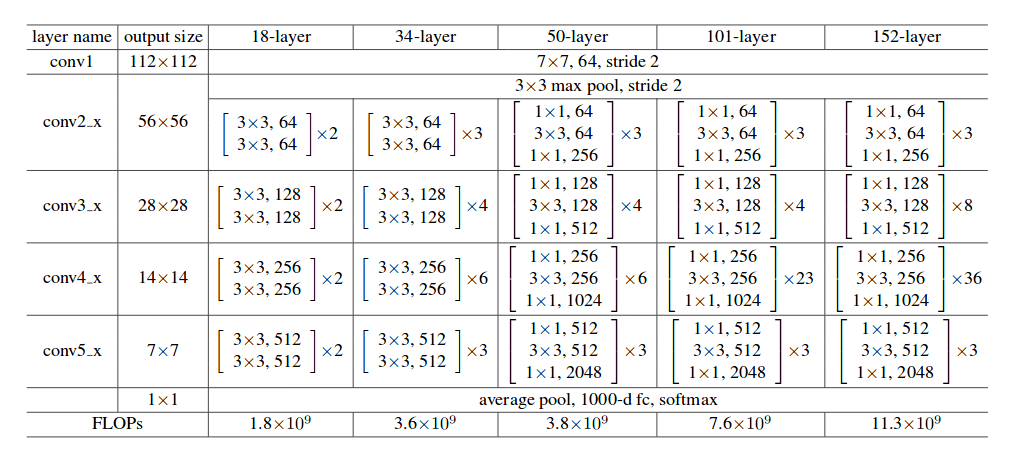
作为两阶段网络的骨干网络，其深度，和性能优劣都深刻的影响着整个网络的性能，其前向推断的速度和准确度都至关重要，VGG作为最原始的骨干网络，各方面的表现都已经落后于新提出的网络。所以我们从Resnet的结构说起

原始VGG网络和Resnet34的对比

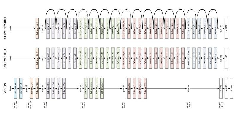
相比VGG的各种问题来说 Resnet提出了新的残差块来对不必要的卷积流程进行跳过，于是网络的加深，高级特征的提取变得更加容易，在此之后，几乎所有的骨干网络更新都是从块结构的优化着手。例如DenseNet就对块结构做出了更多连接模式的探索

简单起见我们从最基础的BackBone-Resnet开始

1，BasicBlock

在代码阶段的表现就是ResNet网络的构建代码中包含了跳层结构

class BasicBlock(nn.Module):
    expansion = 1
    def __init__(self, inplanes, planes, stride=1, downsample=None):
        super(BasicBlock, self).__init__()
        self.conv1 = conv3x3(inplanes, planes, stride)
        self.bn1 = nn.BatchNorm2d(planes)
        self.relu = nn.ReLU(inplace=True)
        self.conv2 = conv3x3(planes, planes)
        self.bn2 = nn.BatchNorm2d(planes)
        self.downsample = downsample
        self.stride = stride

    def forward(self, x):
        identity = x

        out = self.conv1(x)
        out = self.bn1(out)
        out = self.relu(out)

        out = self.conv2(out)
        out = self.bn2(out)

        if self.downsample is not None:
            identity = self.downsample(x)

        out += identity
        out = self.relu(out)
        return out

2.Bottleneck

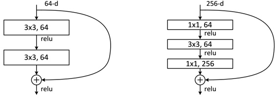
class Bottleneck(nn.Module):
    expansion = 4
    def __init__(self, inplanes, planes, stride=1, downsample=None):
        super(Bottleneck, self).__init__()
        self.conv1 = conv1x1(inplanes, planes)
        self.bn1 = nn.BatchNorm2d(planes)
        self.conv2 = conv3x3(planes, planes, stride)
        self.bn2 = nn.BatchNorm2d(planes)
        self.conv3 = conv1x1(planes, planes * self.expansion)
        self.bn3 = nn.BatchNorm2d(planes * self.expansion)
        self.relu = nn.ReLU(inplace=True)
        self.downsample = downsample
        self.stride = stride

    def forward(self, x):
        identity = x

        out = self.conv1(x)
        out = self.bn1(out)
        out = self.relu(out)

        out = self.conv2(out)
        out = self.bn2(out)
        out = self.relu(out)

        out = self.conv3(out)
        out = self.bn3(out)
        
        if self.downsample is not None:
            identity = self.downsample(x)
        out += identity
        out = self.relu(out)

        return out

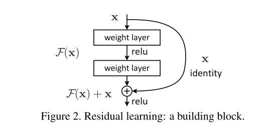
我们在以上网络中看到 跳层的控制结构由 downsample() 控制，也就是说残差块会判断下采样是否为空，如果训练流程执行的不是下采样，那么就进行正常的卷积流程。但是如果训练流程决定执行下采样，就说明残差块中的卷积结果需要加上下采样生成的恒等（identity）。我们从原理上看一下它为什么有效，首先我们来定义残差单元：

其中$h(x)$为identity一般求解过程中直接设为x

$F(x_l,W_l)$为残差函数(w是什么不用说了吧)
$f(x)$为激活函数ReLU
从此定义来看我们从 l 层学习到 L 层：

求反向传播梯度：

表示loss在L层的梯度，小括号里面的是残差梯度，其加法结构相比传统的乘法结构有一个直接的好处就是，可以发现当Loss在很小的时候也因为1的存在不会出现残差梯度的消失，既该层不会像传统网络一样，因为乘法结构导致梯度消失。具体的讨论可以在下面的文章中找到

Identity Mappings in Deep Residual Networks

因为我们只需BackBone作为提取特征的工具， 最终将图片提取为一个合乎其他部分输入的featuremap就可以
我们来看一下，最终的骨干网络怎么构成：

class ResNet(nn.Module):

    def __init__(self, block, layers, num_classes=1000):
        self.inplanes = 64
        super(ResNet, self).__init__()
        self.conv1 = nn.Conv2d(3, 64, kernel_size=7, stride=2, padding=3,
                               bias=False)
        self.bn1 = nn.BatchNorm2d(64)
        self.relu = nn.ReLU(inplace=True)
        self.maxpool = nn.MaxPool2d(kernel_size=3, stride=2, padding=1)
        
        self.layer1 = self._make_layer(block, 64, layers[0])
        self.layer2 = self._make_layer(block, 128, layers[1], stride=2)
        self.layer3 = self._make_layer(block, 256, layers[2], stride=2)
        self.layer4 = self._make_layer(block, 512, layers[3], stride=2)
        
        self.avgpool = nn.AvgPool2d(7, stride=1)
        self.fc = nn.Linear(512 * block.expansion, num_classes)

        for m in self.modules():
            if isinstance(m, nn.Conv2d):
                n = m.kernel_size[0] * m.kernel_size[1] * m.out_channels
                m.weight.data.normal_(0, math.sqrt(2. / n))
            elif isinstance(m, nn.BatchNorm2d):
                m.weight.data.fill_(1)
                m.bias.data.zero_()

    def _make_layer(self, block, planes, blocks, stride=1):
        downsample = None
        if stride != 1 or self.inplanes != planes * block.expansion:
            downsample = nn.Sequential(
                nn.Conv2d(self.inplanes, planes * block.expansion,
                          kernel_size=1, stride=stride, bias=False),
                nn.BatchNorm2d(planes * block.expansion),
            )

        layers = []
        layers.append(block(self.inplanes, planes, stride, downsample))
        self.inplanes = planes * block.expansion
        for i in range(1, blocks):
            layers.append(block(self.inplanes, planes))

        return nn.Sequential(*layers)

    def forward(self, x):
        x = self.conv1(x)
        x = self.bn1(x)
        x = self.relu(x)
        x = self.maxpool(x)

        x = self.layer1(x)
        x = self.layer2(x)
        x = self.layer3(x)
        x = self.layer4(x)

        x = self.avgpool(x)
        x = x.view(x.size(0), -1)
        x = self.fc(x)

        return x

由此生成的标准Resnet肯定是不能为我们直接使用的，因为RPN接口所需要的是FeatureMap不是最后全连接的结果，因此，我们需要Layer3的输出，而不是fc的输出。那么问题来了：

Resnet怎么嫁接到RPN网络呢？

这就要从RPN需要输入的尺寸，和Layer输出的尺寸说起。我们根据图可以看到Resnet101 layer3的输出是1*1,1024

适配工作AnyFeature to RPN

我们以Resnet101为例 来展示一个典型的Resnet 网络作为Faster RCNN的BackBone是怎么一种操作

在原版中,VGG作为BackBone 我们看到的写法是

        self.features = VGG16(bn=False)
        self.conv1 = Conv2d(512, 512, 3, same_padding=True)
        .
        .
        .
   def forward(self, im_data, im_info, gt_boxes=None, gt_ishard=None, dontcare_areas=None):
        features = self.features(im_data)    
        rpn_conv1 = self.conv1(features)

也就是说只要我们把最终把BackBone产生的feature尺寸和Conv1输入的尺寸匹配好就可以了
当我们定义一个Resnet for RPN的类的时候可以参考下面的流程

class resnet(_fasterRCNN):
  def __init__(self, classes, num_layers=101, pretrained=False, class_agnostic=False):
    self.model_path = 'data/pretrained_model/resnet101_caffe.pth'
    self.dout_base_model = 1024
    self.pretrained = pretrained
    self.class_agnostic = class_agnostic

    _fasterRCNN.__init__(self, classes, class_agnostic)

  def _init_modules(self):
    resnet = resnet101()

    if self.pretrained == True:
      print("Loading pretrained weights from %s" %(self.model_path))
      state_dict = torch.load(self.model_path)
      resnet.load_state_dict({k:v for k,v in state_dict.items() if k in resnet.state_dict()})

    # Build resnet.
    ##########################
    self.RCNN_base = nn.Sequential(resnet.conv1, resnet.bn1,resnet.relu,
      resnet.maxpool,resnet.layer1,resnet.layer2,resnet.layer3)

    self.RCNN_top = nn.Sequential(resnet.layer4)
	##########################
    self.RCNN_cls_score = nn.Linear(2048, self.n_classes)
    if self.class_agnostic:
      self.RCNN_bbox_pred = nn.Linear(2048, 4)
    else:
      self.RCNN_bbox_pred = nn.Linear(2048, 4 * self.n_classes)

    # Fix blocks
    for p in self.RCNN_base[0].parameters(): p.requires_grad=False
    for p in self.RCNN_base[1].parameters(): p.requires_grad=False
	
    assert (0 <= cfg.RESNET.FIXED_BLOCKS < 4)
    if cfg.RESNET.FIXED_BLOCKS >= 3:
      for p in self.RCNN_base[6].parameters(): p.requires_grad=False
    if cfg.RESNET.FIXED_BLOCKS >= 2:
      for p in self.RCNN_base[5].parameters(): p.requires_grad=False
    if cfg.RESNET.FIXED_BLOCKS >= 1:
      for p in self.RCNN_base[4].parameters(): p.requires_grad=False

    def set_bn_fix(m):
      classname = m.__class__.__name__
      if classname.find('BatchNorm') != -1:
        for p in m.parameters(): p.requires_grad=False

    self.RCNN_base.apply(set_bn_fix)
    self.RCNN_top.apply(set_bn_fix)

可以看到常见的做法就是把这BackBone分成两部分，以ResNet101为例，这里把构造过程分成了两部分：

self.RCNN_base = nn.Sequential(resnet.conv1, resnet.bn1,resnet.relu,
      resnet.maxpool,resnet.layer1,resnet.layer2,resnet.layer3)

self.RCNN_top = nn.Sequential(resnet.layer4)

  def _head_to_tail(self, pool5):
    fc7 = self.RCNN_top(pool5).mean(3).mean(2)
    return fc7

base_feat = self.RCNN_base(6)

        # feed base feature map tp RPN to obtain rois
rois, rpn_loss_cls, rpn_loss_bbox = self.RCNN_rpn(base_feat, im_info, gt_boxes, num_boxes)

既从最开始到Layer3为一部分，layer4为一部分，在之后的操作中RCNN_Base作为通用的feature输入RPN，而经过ROI Pooling（Align）后的feature进入最后的layer4

        pooled_feat = self.RCNN_roi_pool(base_feat, rois.view(-1,5))
        # ..................最终拼接位置
        pooled_feat = self._head_to_tail(pooled_feat)# compute bbox offset
      

经过layer4之后池化的feature在进入类别预测和box预测 如下:

		# compute bbox offset
        bbox_pred = self.RCNN_bbox_pred(pooled_feat)
        # compute object classification probability
        cls_score = self.RCNN_cls_score(pooled_feat)
        cls_prob = F.softmax(cls_score, 1)

RPN

先看原文怎么描述:

RPN以一个任意尺寸的图像作为输入，输出一组矩形region proposal，每个拥有一个该对象的分数。

最终目标是与 FastR-CNN的检测网络共享计算，我们假设两个网络共享一组共同的转换层。

在原始的设计中BackBone被视为RPN的一部分

在我们的实验中，我们研究了Zeiler和Fergus模型（ZF），它具有5个可共享的卷积层和Simonyan和Zisserman模型（VGG），它具有13个可共享的卷积层。

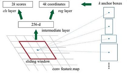
为了生成region proposal，我们对最后一个输出的可分享的卷积层上建立一个小的网络用来滑窗
这个网络完全连接到一个输入卷积特征图的 n*n 空间窗口上。
每个滑窗都被映射到一个更低维的向量中（ZF-256维，VGG512维）

正向量被输入到两个并行的全连接层中

• 框回归分支

• 类回归分支
  

在这篇文章中我们令n=3，实际的感受野在输入图像上非常大，(171 在ZF上 228 在VGG上)。

这个结构天然的以nn卷积层实现并后接两个11的卷积层，ReLUs 被应用在n*n卷积层的输出上。

class RPN(nn.Module):
    _feat_stride = [16, ]
    anchor_scales = [8, 16, 32]

    def __init__(self):
        super(RPN, self).__init__()

        self.features = VGG16(bn=False)
        self.conv1 = Conv2d(512, 512, 3, same_padding=True)
        self.score_conv = Conv2d(512, len(self.anchor_scales) * 3 * 2, 1, relu=False, same_padding=False)
        self.bbox_conv = Conv2d(512, len(self.anchor_scales) * 3 * 4, 1, relu=False, same_padding=False)

        # loss
        self.cross_entropy = None
        self.los_box = None

    @property
    def loss(self):
        return self.cross_entropy + self.loss_box * 10

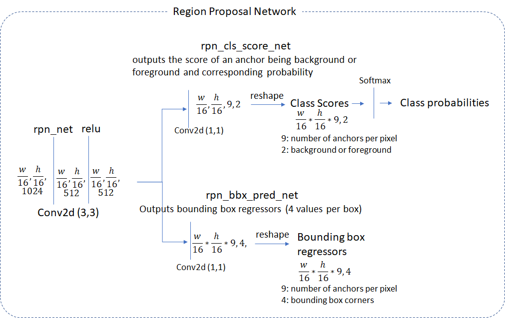
    def forward(self, im_data, im_info, gt_boxes=None, gt_ishard=None, dontcare_areas=None):
            """
                          |-->rpn_cls_score_net--->_______--->Class Scores--->|softmax--->|Class Probabilities
                          |    w/16,h/16,9,2       reshape
                          |  
        rpn_net -->relu-->|
                          |  
                          |-->rpn_bbx_pred_net---->_______--->Bounding Box regressors---->|
                               w/16,h/16,9,4       reshape
        """
        im_data = network.np_to_variable(im_data, is_cuda=True)
        im_data = im_data.permute(0, 3, 1, 2)
        features = self.features(im_data)

        rpn_conv1 = self.conv1(features)

        # rpn cls score net
        rpn_cls_score = self.score_conv(rpn_conv1)
        rpn_cls_score_reshape = self.reshape_layer(rpn_cls_score, 2)
        rpn_cls_prob = F.softmax(rpn_cls_score_reshape)
        rpn_cls_prob_reshape = self.reshape_layer(rpn_cls_prob, len(self.anchor_scales)*3*2)

        # rpn bbx pred net
        rpn_bbox_pred = self.bbox_conv(rpn_conv1)

        # proposal layer
        cfg_key = 'TRAIN' if self.training else 'TEST'
        # 
        rois = self.proposal_layer(rpn_cls_prob_reshape, rpn_bbox_pred, im_info,
                                   cfg_key, self._feat_stride, self.anchor_scales)

        # generating training labels and build the rpn loss
        if self.training:
            assert gt_boxes is not None
            rpn_data = self.anchor_target_layer(rpn_cls_score, gt_boxes, gt_ishard, dontcare_areas,
                                                im_info, self._feat_stride, self.anchor_scales)
            self.cross_entropy, self.loss_box = self.build_loss(rpn_cls_score_reshape, rpn_bbox_pred, rpn_data)

        return features, rois

从原文的途中我们可以体会一下整个流程。输入一张image 输出一组regions proposal
当然其中有些流程需要再解释

Anchor&Proposal layer

执行流程:

for each (H, W) location i

1. 在i位置生成A个anchor box
2. 把预测的包围盒变量应用于每个位置的每个锚点
3. 使用预测盒剪切图片
4. 去掉宽和长小于阈值的包围盒
5. 从高到低对所有proposal，score 序列排序
6. 选择top N 应用 非极大值抑制 使用0.7做阈值

按照Batch返回TopN

既：

• 0.输入之前RPN两条支路中所生成的
  rpn_cls_prob_reshape，
  (1 , H , W , Ax2)
  rpn_bbox_pred，
  (1 , H , W , Ax4)
  以及原始图像的信息
  [image_height, image_width, scale_ratios]
• 1.基于feature map 尺寸，按照指定的长宽大小组合生成所有pixel位置的 anchor（shift_base anchors）
• 2.对这些anchor做剪枝(clip,transfrom,filter,NMS),TopN备选
• 3.把剪枝后的anchor包装为proposal

def proposal_layer(rpn_cls_prob_reshape, rpn_bbox_pred, im_info, cfg_key, _feat_stride=[16, ],
                   anchor_scales=[8, 16, 32]):
    """
    Parameters
    ----------
    rpn_cls_prob_reshape: (1 , H , W , Ax2) outputs of RPN, prob of bg or fg
                         NOTICE: the old version is ordered by (1, H, W, 2, A) !!!!
    rpn_bbox_pred: (1 , H , W , Ax4), rgs boxes output of RPN
    im_info: a list of [image_height, image_width, scale_ratios]
    cfg_key: 'TRAIN' or 'TEST'
    _feat_stride: the downsampling ratio of feature map to the original input image
    anchor_scales: the scales to the basic_anchor (basic anchor is [16, 16])
    ----------
    Returns
    ----------
    rpn_rois : (1 x H x W x A, 5) e.g. [0, x1, y1, x2, y2]

    """
    
    #注意在这个位置就生成了预置框了
    _anchors = generate_anchors(scales=np.array(anchor_scales))
    
    _num_anchors = _anchors.shape[0]
    # rpn_cls_prob_reshape = np.transpose(rpn_cls_prob_reshape,[0,3,1,2]) #-> (1 , 2xA, H , W)
    # rpn_bbox_pred = np.transpose(rpn_bbox_pred,[0,3,1,2])              # -> (1 , Ax4, H , W)

    # rpn_cls_prob_reshape = np.transpose(np.reshape(rpn_cls_prob_reshape,[1,rpn_cls_prob_reshape.shape[0],rpn_cls_prob_reshape.shape[1],rpn_cls_prob_reshape.shape[2]]),[0,3,2,1])
    # rpn_bbox_pred = np.transpose(rpn_bbox_pred,[0,3,2,1])
    im_info = im_info[0]

    assert rpn_cls_prob_reshape.shape[0] == 1, 
        'Only single item batches are supported'
    # cfg_key = str(self.phase) # either 'TRAIN' or 'TEST'
    # cfg_key = 'TEST'
    pre_nms_topN = cfg[cfg_key].RPN_PRE_NMS_TOP_N
    post_nms_topN = cfg[cfg_key].RPN_POST_NMS_TOP_N
    
    #这个阈值很重要
    nms_thresh = cfg[cfg_key].RPN_NMS_THRESH
    
    
    min_size = cfg[cfg_key].RPN_MIN_SIZE

    # the first set of _num_anchors channels are bg probs
    # the second set are the fg probs, which we want
    scores = rpn_cls_prob_reshape[:, _num_anchors:, :, :]
    bbox_deltas = rpn_bbox_pred
    # im_info = bottom[2].data[0, :]

    # 1. Generate proposals from bbox deltas and shifted anchors
    height, width = scores.shape[-2:]


    # Enumerate all shifts
    shift_x = np.arange(0, width) * _feat_stride
    shift_y = np.arange(0, height) * _feat_stride
    shift_x, shift_y = np.meshgrid(shift_x, shift_y)
    shifts = np.vstack((shift_x.ravel(), shift_y.ravel(),
                        shift_x.ravel(), shift_y.ravel())).transpose()

    # Enumerate all shifted anchors:
    #
    # add A anchors (1, A, 4) to
    # cell K shifts (K, 1, 4) to get
    # shift anchors (K, A, 4)
    # reshape to (K*A, 4) shifted anchors
    A = _num_anchors
    K = shifts.shape[0]
    anchors = _anchors.reshape((1, A, 4)) + 
              shifts.reshape((1, K, 4)).transpose((1, 0, 2))
    anchors = anchors.reshape((K * A, 4))

    # Transpose and reshape predicted bbox transformations to get them
    # into the same order as the anchors:
    #
    # bbox deltas will be (1, 4 * A, H, W) format
    # transpose to (1, H, W, 4 * A)
    # reshape to (1 * H * W * A, 4) where rows are ordered by (h, w, a)
    # in slowest to fastest order
    bbox_deltas = bbox_deltas.transpose((0, 2, 3, 1)).reshape((-1, 4))

    # Same story for the scores:
    #
    # scores are (1, A, H, W) format
    # transpose to (1, H, W, A)
    # reshape to (1 * H * W * A, 1) where rows are ordered by (h, w, a)
    scores = scores.transpose((0, 2, 3, 1)).reshape((-1, 1))

    # Convert anchors into proposals via bbox transformations
    proposals = bbox_transform_inv(anchors, bbox_deltas)

    # 2. clip predicted boxes to image
    proposals = clip_boxes(proposals, im_info[:2])

    # 3. remove predicted boxes with either height or width < threshold
    # (NOTE: convert min_size to input image scale stored in im_info[2])
    keep = _filter_boxes(proposals, min_size * im_info[2])
    proposals = proposals[keep, :]
    scores = scores[keep]

    # # remove irregular boxes, too fat too tall
    # keep = _filter_irregular_boxes(proposals)
    # proposals = proposals[keep, :]
    # scores = scores[keep]

    # 4. sort all (proposal, score) pairs by score from highest to lowest
    # 5. take top pre_nms_topN (e.g. 6000)
    order = scores.ravel().argsort()[::-1]
    if pre_nms_topN > 0:
        order = order[:pre_nms_topN]
    proposals = proposals[order, :]
    scores = scores[order]

    # 6. apply nms (e.g. threshold = 0.7)
    # 7. take after_nms_topN (e.g. 300)
    # 8. return the top proposals (-> RoIs top)
    keep = nms(np.hstack((proposals, scores)), nms_thresh)


    if post_nms_topN > 0:
        keep = keep[:post_nms_topN]
    proposals = proposals[keep, :]
    scores = scores[keep]

    # Output rois blob
    # Our RPN implementation only supports a single input image, so all
    # batch inds are 0
    batch_inds = np.zeros((proposals.shape[0], 1), dtype=np.float32)
    blob = np.hstack((batch_inds, proposals.astype(np.float32, copy=False)))
    return blob
    # top[0].reshape(*(blob.shape))
    # top[0].data[...] = blob

    # [Optional] output scores blob
    # if len(top) > 1:
    #    top[1].reshape(*(scores.shape))
    #    top[1].data[...] = scores

Generate Anchors

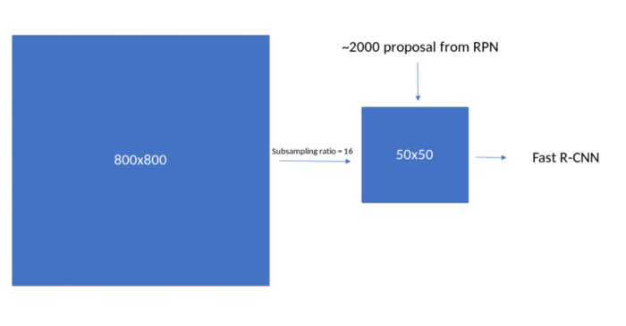
在上一步的proposal layer中我们会发现，anchor的生成过程处于region proposal流程的最前端，那generate到底干了些什么呢？首先从BackBone输入影像，到输出featuremap 由于在取卷积的过程中的一些非padding的操作使得数据层尺寸越来越小，典型的800^2经过VGG下采样后尺寸为
50^2，这个阶段我们先用简单的代码来研究这其中的原理

我们使用
锚点缩放参数8,16,32
长宽比0.5,1,2
下采样倍数为16
现在每个featuremap上的像素都映射了原图1616像素的区域，如上图所示
1.我们首先需要生成在这个1616像素的顶端生成锚点框，然后沿着xy轴去生成所有锚点框

import numpy as np
sub_sample=16
ratio = [0.5, 1, 2]
anchor_scales = [8, 16, 32]
anchor_base = np.zeros((len(ratios) * len(scales), 4), dtype=np.float32)
ctr_y = sub_sample / 2.
ctr_x = sub_sample / 2.
print(ctr_y, ctr_x)
for i in range(len(ratios)):
  for j in range(len(anchor_scales)):
    h = sub_sample * anchor_scales[j] * np.sqrt(ratios[i])
    w = sub_sample * anchor_scales[j] * np.sqrt(1./ ratios[i])
    index = i * len(anchor_scales) + j
    anchor_base[index, 0] = ctr_y - h / 2.
    anchor_base[index, 1] = ctr_x - w / 2.
    anchor_base[index, 2] = ctr_y + h / 2.
    anchor_base[index, 3] = ctr_x + w / 2.
#Out:
# array([[ -37.254833,  -82.50967 ,   53.254833,   98.50967 ],
#        [ -82.50967 , -173.01933 ,   98.50967 ,  189.01933 ],
#        [-173.01933 , -354.03867 ,  189.01933 ,  370.03867 ],
#        [ -56.      ,  -56.      ,   72.      ,   72.      ],
#        [-120.      , -120.      ,  136.      ,  136.      ],
#        [-248.      , -248.      ,  264.      ,  264.      ],
#        [ -82.50967 ,  -37.254833,   98.50967 ,   53.254833],
#        [-173.01933 ,  -82.50967 ,  189.01933 ,   98.50967 ],
#        [-354.03867 , -173.01933 ,  370.03867 ,  189.01933 ]],
#       dtype=float32)

以上的输出为featuremap上第一个像素位置的anchor，我们必须依照这个流程生成所有像素位置上的anchor：

2.在feature map上的每个像素位置，我们需要生成9个锚点框，既每个框由(‘y1’, ‘x1’, ‘y2’, ‘x2’)构成因此总共有95050=22500个框,因此最后，一张图的anchor数据尺寸应该是（22500，4）

3.在22500个框中最后有相当部分的框实质上超出了图像的边界，因此我们根据最直接的边界计算就能筛除，最终22500个框剩下17500个有效框（17500，4）

fe_size = (800//16)
ctr_x = np.arange(16, (fe_size+1) * 16, 16)
ctr_y = np.arange(16, (fe_size+1) * 16, 16)
index = 0
for x in range(len(ctr_x)):
    for y in range(len(ctr_y)):
        ctr[index, 1] = ctr_x[x] - 8
        ctr[index, 0] = ctr_y[y] - 8
        index +=1
 
anchors = np.zeros((fe_size * fe_size * 9), 4)
index = 0
for c in ctr:
  ctr_y, ctr_x = c
  for i in range(len(ratios)):
    for j in range(len(anchor_scales)):
      h = sub_sample * anchor_scales[j] * np.sqrt(ratios[i])
      w = sub_sample * anchor_scales[j] * np.sqrt(1./ ratios[i])
      anchors[index, 0] = ctr_y - h / 2.
      anchors[index, 1] = ctr_x - w / 2.
      anchors[index, 2] = ctr_y + h / 2.
      anchors[index, 3] = ctr_x + w / 2.
      index += 1

print(anchors.shape)
#Out: [22500, 4]

现在我们已经从原理上把所有框都生成了。为了工程调用起见我们用下面的方法包装

def _whctrs(anchor):
    """
    Return width, height, x center, and y center for an anchor (window).
    """

    w = anchor[2] - anchor[0] + 1
    h = anchor[3] - anchor[1] + 1
    x_ctr = anchor[0] + 0.5 * (w - 1)
    y_ctr = anchor[1] + 0.5 * (h - 1)
    return w, h, x_ctr, y_ctr

def _mkanchors(ws, hs, x_ctr, y_ctr):
    """
    Given a vector of widths (ws) and heights (hs) around a center
    (x_ctr, y_ctr), output a set of anchors (windows).
    """

    ws = ws[:, np.newaxis]
    hs = hs[:, np.newaxis]
    anchors = np.hstack((x_ctr - 0.5 * (ws - 1),
                         y_ctr - 0.5 * (hs - 1),
                         x_ctr + 0.5 * (ws - 1),
                         y_ctr + 0.5 * (hs - 1)))
    return anchors

def _ratio_enum(anchor, ratios):
    """
    Enumerate a set of anchors for each aspect ratio wrt an anchor.
    """

    w, h, x_ctr, y_ctr = _whctrs(anchor)
    size = w * h
    size_ratios = size / ratios
    ws = np.round(np.sqrt(size_ratios))
    hs = np.round(ws * ratios)
    anchors = _mkanchors(ws, hs, x_ctr, y_ctr)
    return anchors

def _scale_enum(anchor, scales):
    """
    Enumerate a set of anchors for each scale wrt an anchor.
    """

    w, h, x_ctr, y_ctr = _whctrs(anchor)
    ws = w * scales
    hs = h * scales
    anchors = _mkanchors(ws, hs, x_ctr, y_ctr)
    return anchors

def generate_anchors(base_size=16, ratios=[0.5, 1, 2],
                     scales=2**np.arange(3, 6)):
    """
    Generate anchor (reference) windows by enumerating aspect ratios X
    scales wrt a reference (0, 0, 15, 15) window.
    """

    base_anchor = np.array([1, 1, base_size, base_size]) - 1
    ratio_anchors = _ratio_enum(base_anchor, ratios)
    anchors = np.vstack([_scale_enum(ratio_anchors[i, :], scales)
                         for i in xrange(ratio_anchors.shape[0])])
    return anchors

print(anchors)
#array([[ -83.,  -39.,  100.,   56.],
#       [-175.,  -87.,  192.,  104.],
#       [-359., -183.,  376.,  200.],
#       [ -55.,  -55.,   72.,   72.],
#       [-119., -119.,  136.,  136.],
#       [-247., -247.,  264.,  264.],
#       [ -35.,  -79.,   52.,   96.],
#       [ -79., -167.,   96.,  184.],
#       [-167., -343.,  184.,  360.]])

在实际工程执行的过程中,for循环的操作很慢.因此其实是都以base anchor做shift操作 这部分工作在Region Proposal Layer中可以看到，经过shift产生的所有框就是我们通过简化代码所输出的[22500, 4]得anchors

NMS(Non-Max Suppression)

NMS算法一般是为了去掉模型预测后的多余框，其一般设有一个nms_threshold=0.5，具体的实现思路如下：

选取这类box中scores最大的哪一个，记为box_best，并保留它
计算box_best与其余的box的IOU
如果其IOU>0.5了，那么就舍弃这个box（由于可能这两个box表示同一目标，所以保留分数高的哪一个）
从最后剩余的boxes中，再找出最大scores的哪一个，如此循环往复

---

我们先用最常规的代码去实现nms：

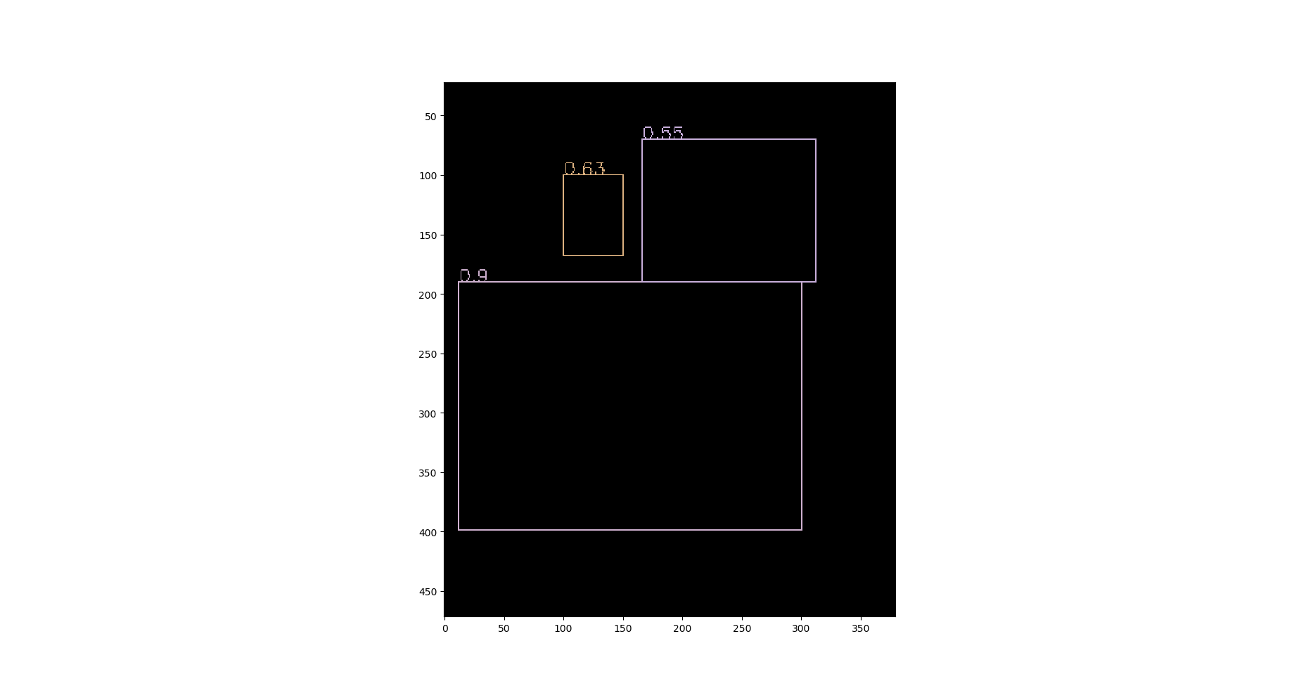
先假设有6个输出的矩形框(即proposal_clip_box)，根据分类器类别分类概率做排序，从小到大分别属于车辆的概率(scores)分别为A、B、C、D、E、F。

(1)从最大概率矩形框F开始，分别判断A~E与F的重叠度IOU是否大于某个设定的阈值;

(2)假设B、D与F的重叠度（IOU）超过阈值，那么就扔掉B、D；并标记第一个矩形框F，是我们保留下来的。

(3)从剩下的矩形框A、C、E中，选择概率最大的E，然后判断E与A、C的重叠度，重叠度大于一定的阈值，那么就扔掉；并标记E是我们保留下来的第二个矩形框。
就这样一直重复，找到所有被保留下来的矩形框。

import numpy as np
import matplotlib.pyplot as plt
import cv2
def display(cordlist):
    back=np.zeros((800,800,3),dtype=np.uint8)
    for index,cord in enumerate(cordlist):
        print('draw ',cord)
        
        color=(np.random.randint(127,255),np.random.randint(127,255),np.random.randint(127,255))
        print('color is ',color)

        cv2.rectangle(back, (int(cord[0]),int(cord[1])), 
        (int(cord[2]),int(cord[3])), color, 1)
        cv2.putText(back, str(cord[4]), (int(cord[0]),int(cord[1])),cv2.FONT_ITALIC,0.5,color, 1)
    plt.imshow(back),plt.show()
    return back



def py_cpu_nms(dets, thresh):
    """Pure Python NMS baseline."""
    # 所有图片的坐标信息，字典形式储存？？
    x1 = dets[:, 0]
    y1 = dets[:, 1]
    x2 = dets[:, 2]
    y2 = dets[:, 3]
    scores = dets[:, 4]

    areas = (x2 - x1 + 1) * (y2 - y1 + 1)  # 计算出所有图片的面积
    order = scores.argsort()[::-1]  # 图片评分按升序排序

    keep = []  # 用来存放最后保留的图片的相应评分
    while order.size > 0:
        i = order[0]  # i 是还未处理的图片中的最大评分
        keep.append(i)  # 保留改图片的值
        # 矩阵操作，下面计算的是图片i分别与其余图片相交的矩形的坐标
        tmp=x1[order[1:]]
        xxxx = x1[i]
        xx1 = np.maximum(x1[i], x1[order[1:]])
        yy1 = np.maximum(y1[i], y1[order[1:]])
        xx2 = np.minimum(x2[i], x2[order[1:]])
        yy2 = np.minimum(y2[i], y2[order[1:]])

        # 计算出各个相交矩形的面积
        w = np.maximum(0.0, xx2 - xx1 + 1)
        h = np.maximum(0.0, yy2 - yy1 + 1)
        inter = w * h
        # 计算重叠比例
        ovr = inter / (areas[i] + areas[order[1:]] - inter)

        # 只保留比例小于阙值的图片，然后继续处理
        inds = np.where(ovr <= thresh)[0]
        indsd= inds+1
        order = order[inds + 1]

    return keep
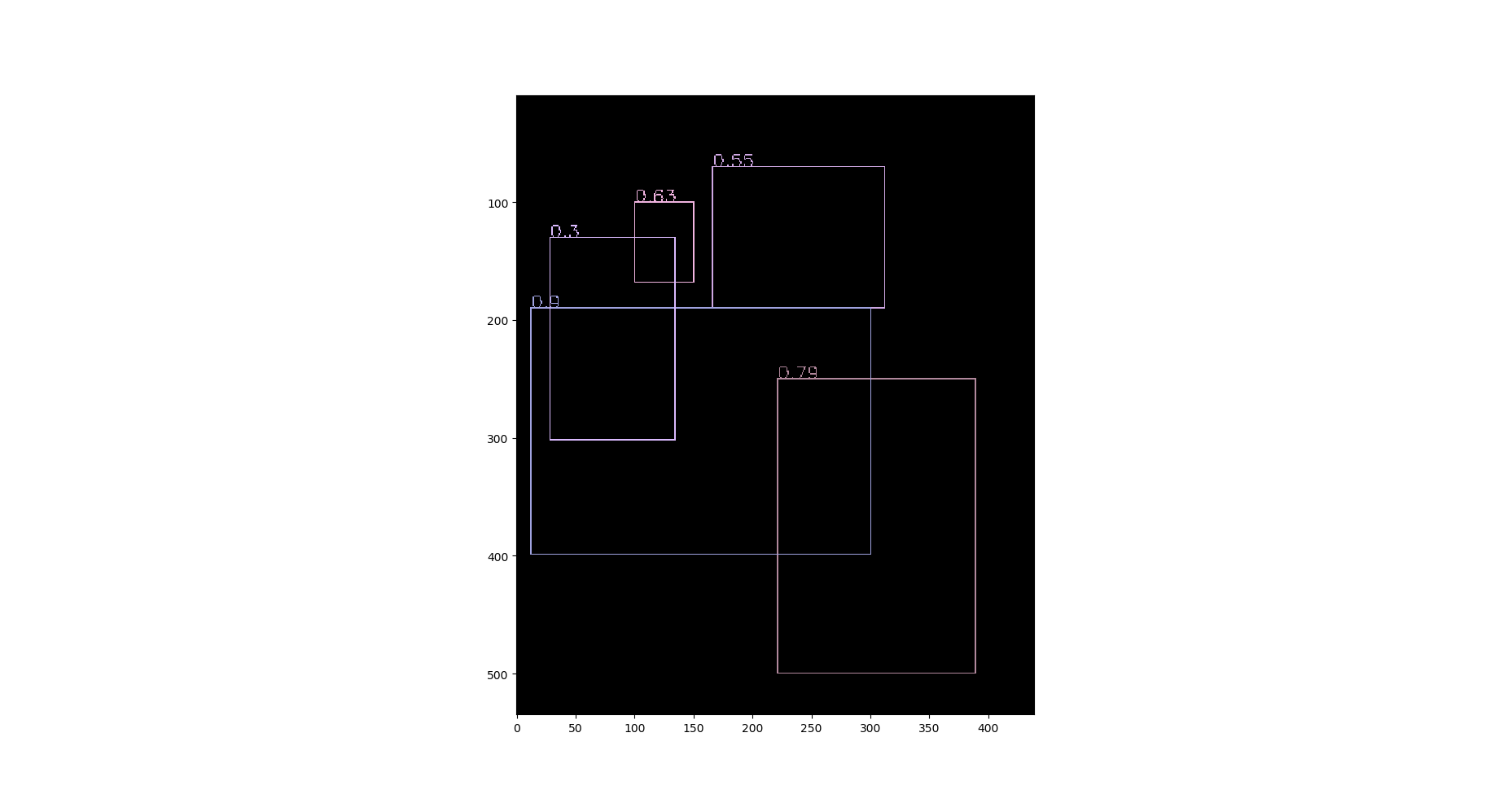
boxes = np.array([[100, 100, 150, 168, 0.63],[166, 70, 312, 190, 0.55],[221, 250, 389, 500, 0.79],[12, 190, 300, 399, 0.9],[28, 130, 134, 302, 0.3]])
# boxes[:,:3]+=100
display(boxes)#显示NMS输入
thresh = 0.1
keep = py_cpu_nms(boxes, thresh)
print('keep:',keep)
keep_=boxes[keep]#nms之后的索引
display(keep_)#显示NMS输出

显示NMS输入

显示NMS输出

有了原理上的了解，我们把整个流程利用torch重构一下

#torch.numel() 表示一个张量总元素的个数
#torch.clamp(min, max) 设置上下限
#tensor.item() 把tensor元素取出作为numpy数字

def nms(self, bboxes, scores, threshold=0.5):
        x1 = bboxes[:,0]
        y1 = bboxes[:,1]
        x2 = bboxes[:,2]
        y2 = bboxes[:,3]
        areas = (x2-x1)*(y2-y1)   # [N,] 每个bbox的面积
        _, order = scores.sort(0, descending=True)    # 降序排列

        keep = []
        while order.numel() > 0:       # torch.numel()返回张量元素个数
            if order.numel() == 1:     # 保留框只剩一个
                i = order.item()
                keep.append(i)
                break
            else:
                i = order[0].item()    # 保留scores最大的那个框box[i]
                keep.append(i)

            # 计算box[i]与其余各框的IOU(思路很好)
            xx1 = x1[order[1:]].clamp(min=x1[i])   # [N-1,]
            yy1 = y1[order[1:]].clamp(min=y1[i])
            xx2 = x2[order[1:]].clamp(max=x2[i])
            yy2 = y2[order[1:]].clamp(max=y2[i])
            inter = (xx2-xx1).clamp(min=0) * (yy2-yy1).clamp(min=0)   # [N-1,]

            iou = inter / (areas[i]+areas[order[1:]]-inter)  # [N-1,]
            idx = (iou <= threshold).nonzero().squeeze() # 注意此时idx为[N-1,] 而order为[N,]
            if idx.numel() == 0:
                break
            order = order[idx+1]  # 修补索引之间的差值
        return torch.LongTensor(keep)   # Pytorch的索引值为LongTensor

经过NMS处理的Proposal，选择TopN个之后
即可被按照Batch返回，结束了整个Region Proposal Layer的过程
Layer返回的Region Proposal以及之前的feature来说 我们已经拿到了RPN网络需要返回的所有信息。可以开始下一步了。

RPN Loss Function

RPN设计完成之后我们来看看Loss函数

RPN Loss计算之前我们先看，原文对于anchor标定的描述

For training RPNs, we assign a binary class label (of being an object or not) to each anchor.
We assign a positive label to two kinds of anchors:

• (i) the anchor/ anchors with the highest Intersection-over-Union (IOU) overlap with a ground-truth box, or
• (ii) an anchor that has an IOU overlap higher than 0.7 with any ground-truth box.

训练RPN网络时，对于每个锚点我们定义了一个二分类标签（是该物体或不是）。
以下两种情况我们视锚点为了一个正样本标签时：

1.锚点和锚点们与标注之间的最高重叠矩形区域	
2.或者锚点和标注的重叠区域指标（IOU）>0.7

Note that a single ground-truth box may assign positive labels to multiple anchors.
Usually the second condition is sufficient to determine the positive samples;

单个正样本的标注框或许被被多个锚点所共享。通常，第二个情况足够可以完成正样本采样。

but we still adopt the first condition for the reason that in some rare cases the
second condition may find no positive sample.

但是我们仍然需要第一种情况，以避免某些少见的情况下，第二种情况下或许会没有正样本采样

We assign a negative label to a non-positive anchor if its IOU ratio is lower than 0.3 for all ground-truth boxes. Anchors that are neither positive nor negative do not contribute to the training objective.

我们给一个非正样本锚点定义负样本标签的时候。如果IOU对所有的标注矩形小于0.3。该锚点将会变成无意义的锚点被过滤掉不会参与训练。

在上一节的定义过程中我们会发现

With these definitions, we minimize an objective function following the multi-task loss in Fast R-CNN
有了这些定义，我们最小化了Fast R-CNN中的多任务损失目标函数。
Our loss function for an image is defined as:
定义为：

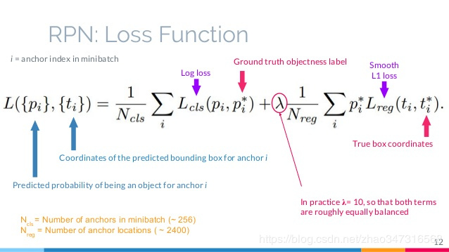
通过该图 我们能从表述和图示里，看出RPN总体loss分为
$$L（P_i,T_i）=L_{cls}+\lambda L_{reg}$$
则在RPN类中可定义为

    @property
    def loss(self):
        return self.cross_entropy + self.loss_box * 10

而与此同时，两种loss的构造还需要执行更多的步骤，其中bbox的loss和类别的交叉熵loss是分别计算的：

    def build_loss(self, rpn_cls_score_reshape, rpn_bbox_pred, rpn_data):
        # classification loss
        rpn_cls_score = rpn_cls_score_reshape.permute(0, 2, 3, 1).contiguous().view(-1, 2)
        rpn_label = rpn_data[0].view(-1)

        rpn_keep = Variable(rpn_label.data.ne(-1).nonzero().squeeze()).cuda()
        rpn_cls_score = torch.index_select(rpn_cls_score, 0, rpn_keep)
        rpn_label = torch.index_select(rpn_label, 0, rpn_keep)

        fg_cnt = torch.sum(rpn_label.data.ne(0))

        rpn_cross_entropy = F.cross_entropy(rpn_cls_score, rpn_label)

        # box loss
        rpn_bbox_targets, rpn_bbox_inside_weights, rpn_bbox_outside_weights = rpn_data[1:]
        rpn_bbox_targets = torch.mul(rpn_bbox_targets, rpn_bbox_inside_weights)
        rpn_bbox_pred = torch.mul(rpn_bbox_pred, rpn_bbox_inside_weights)

        rpn_loss_box = F.smooth_l1_loss(rpn_bbox_pred, rpn_bbox_targets, size_average=False) / (fg_cnt + 1e-4)

        return rpn_cross_entropy, rpn_loss_box

通过以上的loss构造完成了两部分rpn_cross_entropy, rpn_loss_box这两个部分共同构成了RPN_Loss

当能够正常反向传播之后我们应当能够认识到，训练流程里RPN的阶段就彻底结束了。
RPN生成的feature & region proposals

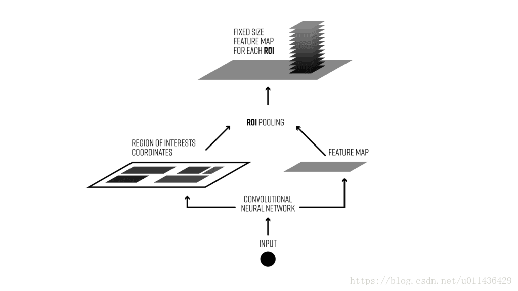
ROI-Pooling

为什么需要ROI Pooling？？
它和我们遇到的MaxPooling，MeanPooling，Sptial Pyramaid Pooling有什么不同？

目标检测2 stage typical architecture 通常可以分为两个阶段：

• （1）region proposal：给定一张输入image找出objects可能存在的所有位置。这一阶段的输出应该是一系列object可能位置的bounding box。（regions or ROIs）

• （2）final classification：确定上一阶段的每个region proposal是否属于目标类别或者背景。

也就是proposal到refine的整体流程

ROI Pooling的目的就是使用MaxPooling针对不定尺寸的输入，产生指定尺寸的feature map。

这个architecture存在的一些问题是：

1，产生大量的region proposals 会导致性能问题，实时性能会大大降低
2，在处理速度方面是suboptimal。
3，无法做到端到端的训练

由于这个步骤没有得到大多数神经网络库的支持，所以需要实现足够快的ROI Pooling操作，这就需要使用C来执行，在GPU条件下需要CUDA来执行

ROI pooling具体操作如下：
（1）根据输入image，将ROI映射到feature map对应位置；
（2）将映射后的区域划分为相同大小的sections（sections数量与输出的维度相同）；
（3）对每个sections进行max pooling操作；
这样我们就可以从不同大小的方框得到固定大小的相应 的feature maps。值得一提的是，输出的feature maps的大小不取决于ROI和卷积feature maps大小。ROI pooling 最大的好处就在于极大地提高了处理速度。
如下图所示：

以下为一个 ROI pooling 的例子
考虑一个8×8大小的feature map，一个ROI，以及输出大小为2×2.
（1）输入的固定大小的 feature map
（2）region proposal 投影之后位置（左上角，右下角坐标）：（0，3），（7，8）。
（3）将其划分为（2×2）个sections（因为输出大小为2×2），我们可以得到：
（4）对每个section做max pooling，可以得到：

class RoIPoolFunction(Function):
    def __init__(self, pooled_height, pooled_width, spatial_scale):
        self.pooled_width = int(pooled_width)
        self.pooled_height = int(pooled_height)
        
        self.spatial_scale = float(spatial_scale)
        self.output = None
        self.argmax = None
        self.rois = None
        self.feature_size = None

    def forward(self, features, rois):
        batch_size, num_channels, data_height, data_width = features.size()
        num_rois = rois.size()[0]
        output = torch.zeros(num_rois, num_channels, self.pooled_height, self.pooled_width)
        argmax = torch.IntTensor(num_rois, num_channels, self.pooled_height, self.pooled_width).zero_()

        if not features.is_cuda:
            _features = features.permute(0, 2, 3, 1)
            roi_pooling.roi_pooling_forward(self.pooled_height, self.pooled_width, self.spatial_scale,
                                            _features, rois, output)
            # output = output.cuda()
        else:
            output = output.cuda()
            argmax = argmax.cuda()
            roi_pooling.roi_pooling_forward_cuda(self.pooled_height, self.pooled_width, self.spatial_scale,
                                                 features, rois, output, argmax)
            self.output = output
            self.argmax = argmax
            self.rois = rois
            self.feature_size = features.size()

        return output

    def backward(self, grad_output):
        assert(self.feature_size is not None and grad_output.is_cuda)

        batch_size, num_channels, data_height, data_width = self.feature_size

        grad_input = torch.zeros(batch_size, num_channels, data_height, data_width).cuda()
        roi_pooling.roi_pooling_backward_cuda(self.pooled_height, self.pooled_width, self.spatial_scale,
                                              grad_output, self.rois, grad_input, self.argmax)

        # print grad_input

        return grad_input, None

可以看到ROI Pooling的 Python 部分其实没有什么计算的部分，其计算部分都被隐藏在了CUDA-C以及C中，以保证其高效。
我们对比一下C和CUDA的代码(forward)
CUDA:

int roi_pooling_forward_cuda(int pooled_height, int pooled_width, float spatial_scale,
                        THCudaTensor * features, THCudaTensor * rois, THCudaTensor * output, THCudaIntTensor * argmax)
{
    // Grab the input tensor
    float * data_flat = THCudaTensor_data(state, features);//输入的Featuremap
    float * rois_flat = THCudaTensor_data(state, rois);//输入的多个ROI

    float * output_flat = THCudaTensor_data(state, output);
    int * argmax_flat = THCudaIntTensor_data(state, argmax);

    // Number of ROIs
    int num_rois = THCudaTensor_size(state, rois, 0);//ROI的数量
    int size_rois = THCudaTensor_size(state, rois, 1);//ROI的尺寸
    if (size_rois != 5)
    {
        return 0;
    }

    // batch size
    int batch_size = THCudaTensor_size(state, features, 0);
    if (batch_size != 1)
    {
        return 0;
    }
    // data height
    int data_height = THCudaTensor_size(state, features, 2);
    // data width
    int data_width = THCudaTensor_size(state, features, 3);
    // Number of channels
    int num_channels = THCudaTensor_size(state, features, 1);

    cudaStream_t stream = THCState_getCurrentStream(state);

    ROIPoolForwardLaucher(
        data_flat, spatial_scale, num_rois, data_height,
        data_width, num_channels, pooled_height,
        pooled_width, rois_flat,
        output_flat, argmax_flat, stream);

    return 1;
}

在这段代码中所有数据被整合进了ROIPoolForwardLauncher中，然后执行了

int ROIPoolForwardLaucher(
    const float* bottom_data, const float spatial_scale, const int num_rois, const int height,
    const int width, const int channels, const int pooled_height,
    const int pooled_width, const float* bottom_rois,
    float* top_data, int* argmax_data, cudaStream_t stream)
{
    const int kThreadsPerBlock = 1024;
    const int output_size = num_rois * pooled_height * pooled_width * channels;
    cudaError_t err;

	在此执行真正的forward计算
    ROIPoolForward<<<(output_size + kThreadsPerBlock - 1) / kThreadsPerBlock, kThreadsPerBlock, 0, stream>>>(
      output_size, bottom_data, spatial_scale, height, width, channels, pooled_height,
      pooled_width, bottom_rois, top_data, argmax_data);
	
    err = cudaGetLastError();
    if(cudaSuccess != err)
    {
        fprintf( stderr, "cudaCheckError() failed : %sn", cudaGetErrorString( err ) );
        exit( -1 );
    }

    return 1;
}

真正的ROI Pooling Forward Kernal 计算：

__global__ void ROIPoolForward(const int nthreads, const float* bottom_data,
    const float spatial_scale, const int height, const int width,
    const int channels, const int pooled_height, const int pooled_width,
    const float* bottom_rois, float* top_data, int* argmax_data)
{
    CUDA_1D_KERNEL_LOOP(index, nthreads)
    {
        // (n, c, ph, pw) is an element in the pooled output
        int n = index;
        int pw = n % pooled_width;
        n /= pooled_width;
        int ph = n % pooled_height;
        n /= pooled_height;
        int c = n % channels;
        n /= channels;

        bottom_rois += n * 5;
        int roi_batch_ind = bottom_rois[0];
        int roi_start_w = round(bottom_rois[1] * spatial_scale);
        int roi_start_h = round(bottom_rois[2] * spatial_scale);
        int roi_end_w = round(bottom_rois[3] * spatial_scale);
        int roi_end_h = round(bottom_rois[4] * spatial_scale);

        // Force malformed ROIs to be 1x1
        int roi_width = fmaxf(roi_end_w - roi_start_w + 1, 1);
        int roi_height = fmaxf(roi_end_h - roi_start_h + 1, 1);
        float bin_size_h = (float)(roi_height) / (float)(pooled_height);
        float bin_size_w = (float)(roi_width) / (float)(pooled_width);

        int hstart = (int)(floor((float)(ph) * bin_size_h));
        int wstart = (int)(floor((float)(pw) * bin_size_w));
        int hend = (int)(ceil((float)(ph + 1) * bin_size_h));
        int wend = (int)(ceil((float)(pw + 1) * bin_size_w));

        // Add roi offsets and clip to input boundaries
        hstart = fminf(fmaxf(hstart + roi_start_h, 0), height);
        hend = fminf(fmaxf(hend + roi_start_h, 0), height);
        wstart = fminf(fmaxf(wstart + roi_start_w, 0), width);
        wend = fminf(fmaxf(wend + roi_start_w, 0), width);
        bool is_empty = (hend <= hstart) || (wend <= wstart);

        // Define an empty pooling region to be zero
        float maxval = is_empty ? 0 : -FLT_MAX;
        // If nothing is pooled, argmax = -1 causes nothing to be backprop'd
        int maxidx = -1;
        bottom_data += roi_batch_ind * channels * height * width;
        for (int h = hstart; h < hend; ++h) {
            for (int w = wstart; w < wend; ++w) {
    //            int bottom_index = (h * width + w) * channels + c;
                int bottom_index = (c * height + h) * width + w;
                if (bottom_data[bottom_index] > maxval) {
                    maxval = bottom_data[bottom_index];
                    maxidx = bottom_index;
                }
            }
        }
        top_data[index] = maxval;
        if (argmax_data != NULL)
            argmax_data[index] = maxidx;
    }
}

有了CUDA的加速RoiPooling的执行过程就变得快了很多，所以突破了端到端的ROI-Pooling的效率问题。Faster RCNN的效率才破除了最后一个障碍

但是实质上，以上过程里展现的信息，在工程上是没有必要的，为任何一个API编写CUDA扩展的难度都是非常大的甚至1%

Regression

在最之前的Faster R-CNN的代码中我们看到了在ROI Pooling之后的过程如下（省略了不必要的部分）

class Faster_RCNN(nn.Module)
    def __init__(self, classes=None, debug=False):
        super(FasterRCNN, self).__init__()
		# roi pooling 之前的定义部分省略

        if classes is not None:
            self.classes = classes
            self.n_classes = len(classes)

        self.rpn = RPN()
        self.roi_pool = RoIPool(7, 7, 1.0/16)
        self.fc6 = FC(512 * 7 * 7, 4096)
        self.fc7 = FC(4096, 4096)
        self.score_fc = FC(4096, self.n_classes, relu=False)
        self.bbox_fc = FC(4096, self.n_classes * 4, relu=False)


    def forward(self, im_data, im_info, gt_boxes=None, gt_ishard=None, dontcare_areas=None):
    
    ......roi之前的部分省略

        pooled_features = self.roi_pool(features, rois)


        x = pooled_features.view(pooled_features.size()[0], -1)
        x = self.fc6(x)
        x = F.dropout(x, training=self.training)
        x = self.fc7(x)
        x = F.dropout(x, training=self.training)

        cls_score = self.score_fc(x)
        cls_prob = F.softmax(cls_score)
        bbox_pred = self.bbox_fc(x)
        
        return cls_prob, bbox_pred, rois

到达了这一步，最终我们实现了整个网络从输入图片数据，到输出预测框以及类别信息的整个流程

Faster RCNN Loss

我们有了两个网络,即Faster RCNN以及RPN,他们也有两个输出 (回归部分以及分类部分),而Faster RCNN的Loss可以定义为:

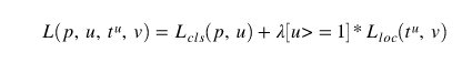
    def build_loss(self, cls_score, bbox_pred, roi_data):
        # classification loss
        label = roi_data[1].squeeze()
        fg_cnt = torch.sum(label.data.ne(0))
        bg_cnt = label.data.numel() - fg_cnt

        # for log
        if self.debug:
            maxv, predict = cls_score.data.max(1)
            self.tp = torch.sum(predict[:fg_cnt].eq(label.data[:fg_cnt])) if fg_cnt > 0 else 0
            self.tf = torch.sum(predict[fg_cnt:].eq(label.data[fg_cnt:]))
            self.fg_cnt = fg_cnt
            self.bg_cnt = bg_cnt

        ce_weights = torch.ones(cls_score.size()[1])
        ce_weights[0] = float(fg_cnt) / bg_cnt
        ce_weights = ce_weights.cuda()
        cross_entropy = F.cross_entropy(cls_score, label, weight=ce_weights)

        # bounding box regression L1 loss
        bbox_targets, bbox_inside_weights, bbox_outside_weights = roi_data[2:]
        bbox_targets = torch.mul(bbox_targets, bbox_inside_weights)
        bbox_pred = torch.mul(bbox_pred, bbox_inside_weights)

        loss_box = F.smooth_l1_loss(bbox_pred, bbox_targets, size_average=False) / (fg_cnt + 1e-4)

        return cross_entropy, loss_box

最终整个loss如下

    @property
    def loss(self):
        return self.cross_entropy + self.loss_box * 10

最后带上了Loss我们看一下

graph TB

subgraph Data preprocess
Dataset -->|transfrom|ROIDatalayer
ROIDatalayer --> |dataloader|minibatch
end
minibatch --> |BackBone|Featuremaps
minibatch--> GtBox

subgraph RPN layer
Featuremaps-->|conv1|Featureconv1
Featureconv1-->|score_conv1|RPN_CLS_prob
Featureconv1-->|bbox_conv1|RPN_BBox_pred
RPN_CLS_prob-->|Proposal_layer / reshape/ softmax| ROIS
RPN_BBox_pred-->|Proposal_layer| ROIS
end

subgraph Loss
GtBox-->|anchor_target_layer|rpn_data
RPN_CLS_prob-->|anchor_target_layer|rpn_data
rpn_data-->rpn_loss
RPN_CLS_prob-->rpn_loss
RPN_BBox_pred-->rpn_loss
ROIS-->|proposal_target_layer|roi_data
GtBox-->|proposal_target_layer|roi_data
bbox_pred-->Netloss
cls_prob-->Netloss
roi_data-->Netloss
Netloss-->Loss
rpn_loss-->Loss
end



subgraph ROI layer
Featuremaps-->|Roi pooling|features_pooled
ROIS-->|Roi pooling|features_pooled

end

subgraph Regression&Classifier
features_pooled-->|view|FC6
FC6-->|dp|FC7
FC7-->|dp+score_fc|cls_score
cls_score-->|Softmax|cls_prob
FC7-->|bbox_fc|bbox_pred

end

最后

以上就是坚强篮球为你收集整理的可能是史上最详细-Faster RCNN Pytorch 复现全纪录的全部内容，希望文章能够帮你解决可能是史上最详细-Faster RCNN Pytorch 复现全纪录所遇到的程序开发问题。

如果觉得靠谱客网站的内容还不错，欢迎将靠谱客网站推荐给程序员好友。