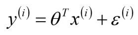
线性回归模型表达式:
- 其中theta.shape=(1,m),m=数据的特征数量。
- 通过直接求导,可以得到theta的最优解,但是会遇到矩阵求逆的问题,而并不是所有的矩阵都可以求逆。
- 由于矩阵求逆的不确定性,因而想到了用梯度下降法来逐步逼近最优解,梯度下降法又分为BGD、SGD、MBGD。
- BGD每次更新需要用全部数据,计算量大且耗时;SGD每次更新需要用一条数据,计算量小速度快,但是可能在最小值附近波动,不收敛;MBGD每次更新用一部分数据(batch_size),计算速度并不会比SGD慢太多,每次使用一个batch_size可以大大减小收敛所需要的迭代次数。
- batch_size根据GPU来选择,一般是32的倍数。
#coding=utf-8
import pandas as pd
import numpy as np
import matplotlib.pyplot as plt
from sklearn import linear_model

np.random.seed(4)

class LR:
    def __init__(self,iter_n=30,learn_rate=0.001,batch_size=2):
        self.iter_n = iter_n
        self.learn_rate = learn_rate
        self.batch_size = batch_size

    #线性回归算法模型:theta*x
    def model(self,x,theta):
        return np.dot(x,theta)

    #损失函数(目标函数):选用MSE均方误差
    def mse(self,y,y_hat):
        return sum((y-y_hat)**2)/len(y)

    #计算梯度
    def cal_gred(self,y,y_hat,x):
        #初始化梯度
        gred = np.zeros((x.shape[-1],1))
        #计算每个theta的梯度
        for index in range(len(gred)):
            gred[index][0] = sum((y-y_hat)*x[:,index:index+1])   #损失通过推倒发现是最小二乘法表达式,再求导就是这个式子
        return gred

    #打乱数据
    def shuffle(self,x,y,y_hat):
        all_data = np.hstack((x,y,y_hat))
        print(all_data)
        np.random.shuffle(all_data)
        return all_data[:,:x.shape[-1]],all_data[:,x.shape[-1]:x.shape[-1]+1],all_data[:,-1:]

    #画损失曲线
    def draw_loss(self,count,loss):
        plt.plot(range(count+1),loss,color='r',marker='o')
        plt.show()

    #对新数据预测
    def predict(self,x):
        x.insert(0,1)
        x = np.array(x)
        y_pre = self.model(x,self.theta)
        #print(y_pre)
        return y_pre

    #拟合
    def fit(self,x,y):
        #训练数据增加一列1,因为theta有偏置项
        x_ones = np.ones((len(x),1))
        x = np.hstack((x_ones,x))
        #初始化theta,初始值设为0
        theta = np.zeros((x.shape[-1],1))  #theta.shape=(4,1)
        #计算预测值(第一次)
        y_hat = self.model(x,theta)
        #计算损失(第一次)
        loss = []
        loss.append(self.mse(y,y_hat))
        #记录迭代次数
        count = 0
        while True:
            #训练一轮(epoh)数据
            for n in range(int(len(x)/self.batch_size)):
                gred = self.cal_gred(y[n*self.batch_size:(n+1)*self.batch_size],y_hat[n*self.batch_size:(n+1)*self.batch_size],x[n*self.batch_size:(n+1)*self.batch_size])
                theta = theta+self.learn_rate*gred
                y_hat = self.model(x,theta)
                loss.append(self.mse(y,y_hat))
                count += 1

            #停止条件 方式1 (用迭代次数控制)
            if count >= self.iter_n:
                #print(f'停止条件为方式1,迭代次数count={count}')
                break

            #停止条件 方式2 (用损失不再降低来控制)
            if loss[-2]-loss[-1] < 1e-5:
                #print(f'停止条件为方式2,迭代次数count={count}')
                break

            #一轮数据全部使用完后,打乱
            x,y,y_hat = self.shuffle(x,y,y_hat)

        self.draw_loss(count,loss)
        self.theta = theta

if __name__=='__main__':
    train_data = pd.read_excel('lr.xlsx',sheet_name='训练数据')   #train_data.shape=(10,4)
    train_data_x = np.array(train_data.iloc[:,:-1])              #train_data_x.shape=(10,3)
    train_data_y = np.array(train_data.iloc[:,-1:])              #train_data_y.shape=(10,1)

    #手写代码结果
    print('------手写结果:以下是手写的线性回归模型结果------')
    lr1 = LR(iter_n=30, learn_rate=0.001, batch_size=4)
    lr1.fit(train_data_x, train_data_y)
    print('预测值为:',lr1.predict([2,4,3]))            #根据拟合的模型,对数据[2,4,3]进行预测,y_hat=1.76261384
    print('截距+权重:',lr1.theta.T)  # y = theta0*1 + theta1*x1 + theta2*x2 + theta3*x3
    # [[theta0 theta1 theta2 theta3]] = [[0.03055664 0.24267117 0.15796392 0.20495306]]

    #调包结果
    print('------调包结果:以下调用sklearn中线性回归模型结果------')
    lr2 = linear_model.LinearRegression()
    lr2.fit(train_data_x, train_data_y)  # y = intercept_ + theta1*x1 + theta2*x2 + theta3*x3
    print('预测值为:',lr2.predict(np.array([[2,4,3]])))   #根据拟合的模型,对数据[2,4,3]进行预测,y_hat=1.62696405
    print('权重:',lr2.coef_)                 # 特征前的系数(权重):[[theta1 theta2 theta3]] = [[0.19642699 0.35235242 0.31708833]]
    print('截距:',lr2.intercept_)            # 截距:[intercept_] = [-1.12656458]
注:lr.xlsx数据是随便写的,不具有参考价值
| x1 | x2 | x3 | y |
|---|---|---|---|
| 2 | 4 | 3 | 1.3 |
| 3 | 4 | 3 | 2.3 |
| 4 | 5 | 6 | 3.4 |
| 5 | 5 | 0 | 2.1 |
| 6 | 4 | 3 | 1 |
| 7 | 4 | 7 | 5 |
| 8 | 3 | 7 | 4.5 |
| 9 | 4 | 7 | 3 |
| 10 | 7 | 7 | 4 |
| 11 | 7 | 6 | 7 |
最后
以上就是敏感犀牛最近收集整理的关于机器学习算法:线性回归 - MBGD小批量梯度下降法 - 手写代码的全部内容,更多相关机器学习算法:线性回归内容请搜索靠谱客的其他文章。
本图文内容来源于网友提供,作为学习参考使用,或来自网络收集整理,版权属于原作者所有。


发表评论 取消回复