matlab中step_Matlab-自动化控制系统设计2时域分析

本文内容：系统的时域分析

操作环境：matlab2019b

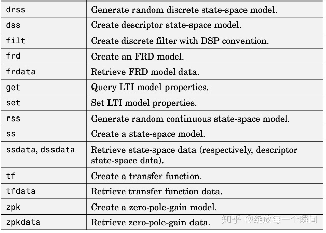
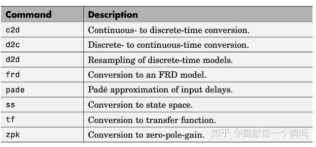
最近小编找到了一个构建控制系统模型的函数列表，感觉还是很全的，先分享一下~

好了，言归正传，我们来说一下时域分析吧，在自控系统中，科学家们给系统一个典型的输入信号（一般为阶跃信号），然后根据响应的表达式和时间响应曲线来分析系统性能，例如稳定性、快速性、平稳性、准确性等等，这就是时间响应分析。接下来，小编将介绍MATLAB中的三种分析方法：编程法，ltiview工具箱以及simulink。

一、编程法：

主要函数：step

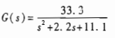
例如以上的传递函数

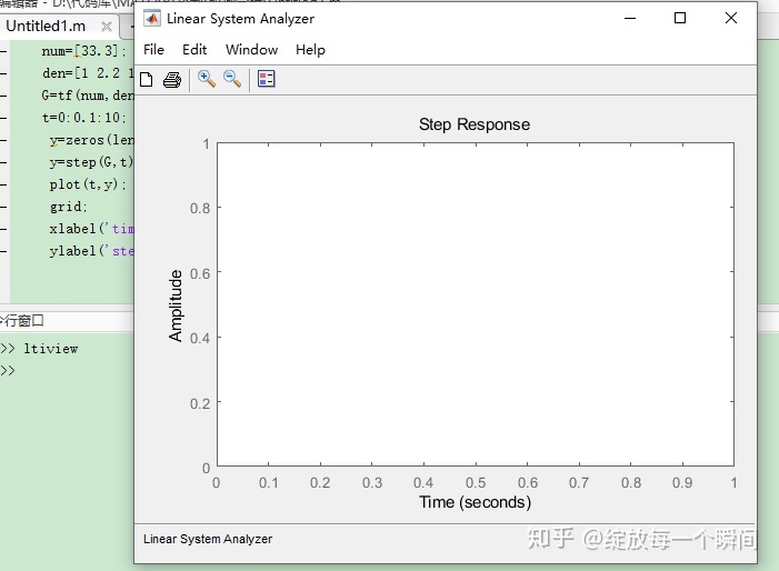
num=[33.3];
den=[1 2.2 11.1];
G=tf(num,den);
%建立传递函数模型
t=0:0.1:10;
%设置时间间隔
y=zeros(length(t));
%创建全0数组存放输出
y=step(G,t);
%输出阶跃相应
plot(t,y);
%作图
grid;
xlabel('time(s)');
ylabel('step response');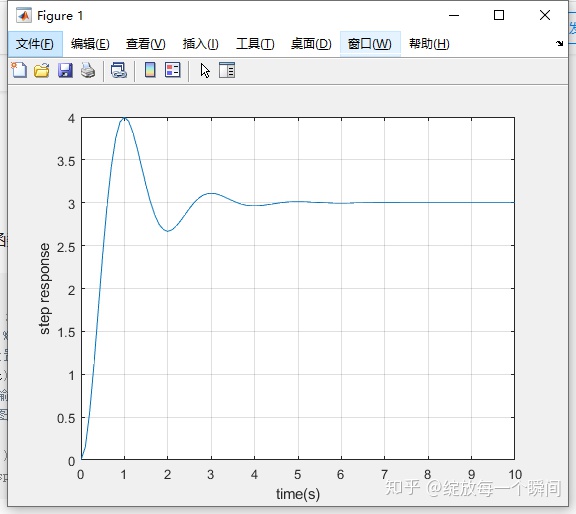

得到以上图像，这里的纵坐标的分度值是系统适应输出响应自动生成的

要想得到超调量、调节时间等指标，可以通过拖动鼠标测量得到，也可以对y编程实现，毕竟这里的输出y是一个数组，大家感兴趣可以自行摸索一下。小编这里介绍另外的两个工具可以方便的得到超调量、调节时间等等。

二、ltiview工具箱：

首先解释一下LIT系统，LIT是线性时不变系统（liner，time-invariable system）的缩写，也就是常说的线性定常系统，matlab为此设计了对应的ltiview工具包。

在命令行窗口输入

ltiview

即可调用该工具包

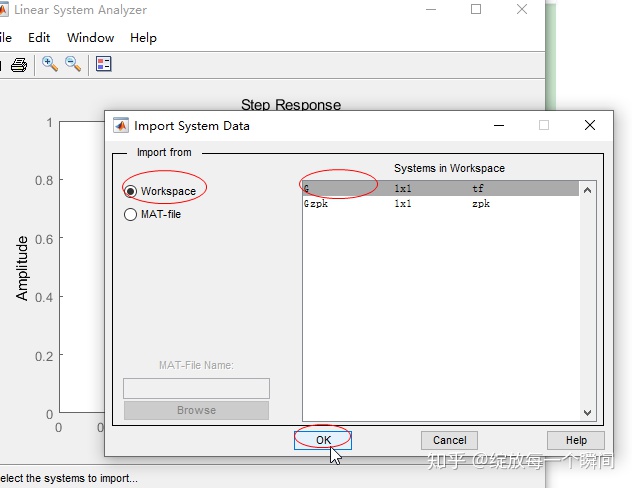
选择File-inport，选择刚刚建立的传递函数G，即可得到相应曲线。

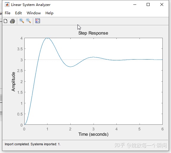
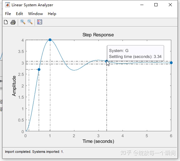
然后右击空白处，选择characteristic- 即可在图像中标出峰值点、稳态点等。鼠标拖动到这些点上就可以看见超调量、调节时间等性能指标了~

三、simulink工具箱：

使用simulink工具箱就可以在scop模块里查看了，不过需要重新搭建一个传递函数。

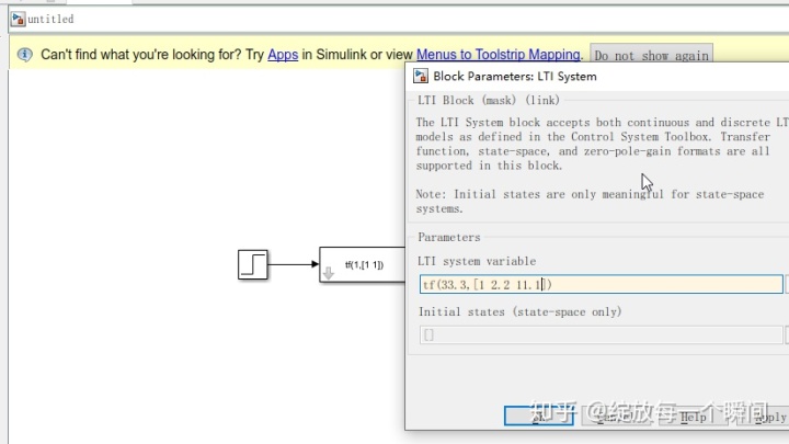
可以选择control system toolbox里的LTI system

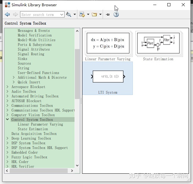
设置好参数和输入模块step和测量模块scope

运行一下

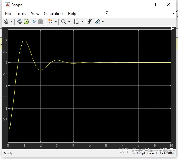
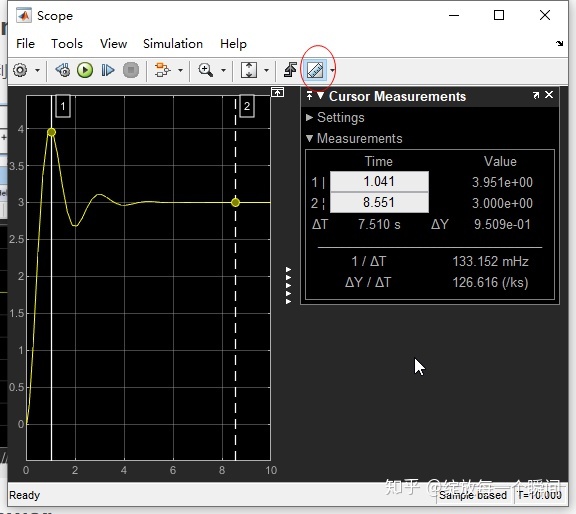
然后运用scope里人游标来测量就OK了~

本文为小编自行编程，如有错误还请大家批评指出~

待更新~下一篇为“matlab中的根轨迹和频域分析法”