序
原来都是用的c++学习的传统图像分割算法。主要学习聚类分割、水平集、图割,欢迎一起讨论学习。
刚刚开始学习cs231n的课程,正好学习python,也做些实战加深对模型的理解。
课程链接
1、这是自己的学习笔记,会参考别人的内容,如有侵权请联系删除。
2、有些原理性的内容不会讲解,但是会放上我觉得讲的不错的博客链接
3、由于之前没怎么用过numpy,也对python不熟,所以也是一个python和numpy模块的学习笔记
本章前言:本章主要对使用tensorflow搭建一个卷积神经网络的流程进行讲述,以后的学习也会使用tensorflow以及keras。有些方法定义在之前的文章中已经讲过了tensorflow的基本内容
import tensorflow as tf
import numpy as np
import math
import timeit
from data_utils import load_cifar10
import matplotlib.pyplot as plt
%matplotlib inline
#自动加载外部模块
%reload_ext autoreload
%autoreload 2
1、读取cifar10图像
读取cifar10图像在之前的博客中也讲述过,这边不再多讲
def get_cifar_data(num_training =49000,num_validation=1000,num_test=10000):
    X_train,y_train,X_test,y_test = load_cifar10('cifar-10-batches-py')
    #验证集
    mask = range(num_training, num_training+num_validation)     #先取验证集,大小为最后的1000条数据
    X_val = X_train[mask]
    y_val = y_train[mask]
    #训练集
    mask = range(num_training)
    X_train = X_train[0:num_training,:,:,:]
    y_train = y_train[mask]
    #测试集
    mask = range(num_test)
    X_test = X_test[mask]
    y_test = y_test[mask]

    mean_image = np.mean(X_train, axis=0)
    #归一化操作,将所有的特征都减去对应的均值
    X_train -= mean_image
    X_val -= mean_image
    X_test -= mean_image

    return X_train,y_train,X_val,y_val,X_test,y_test
X_train,y_train,X_val,y_val,X_test,y_test = get_cifar_data()
print('Train data shape: ', X_train.shape)
print('Train labels shape: ', y_train.shape)
print("validation data shape: ", X_val.shape)
print('validation labels shape: ', y_val.shape)
print('test data shape: ', X_test.shape)
print('test labels shape: ',y_test.shape)
"""
Train data shape: (49000, 32, 32, 3)
Train labels shape: (49000,)
validation data shape: (1000, 32, 32, 3)
validation labels shape: (1000,)
test data shape: (10000, 32, 32, 3)
test labels shape: (10000,)
"""2、tensorflow搭建简单模型
在tensorflow中搭建神经网络只需要完成向前传播的部分,反向传播是由框架完成的,当然反向传播原理还是要理解的。
simple_model搭建的是卷积网络中向前传播的部分,结构为input -> conv1 -> relu -> full-connect
1、卷积运用的是tf.nn.conv2d,stride为步长,第4维和第1维必须为1,padding只有‘VALID’和SAME两个属性
2、激活用的是tf.nn.relu完成relu激活
3、tf.matmul()是矩阵相乘,tf.multiply()是对应位置相乘
4、定义完向前传播,那么我们的输出y_out就有了,有了y_out我们才能计算损失值
损失值的计算利用框架完成:tf.loss.hinge_loss(),是svm中使用的损失函数。
5、我们的目标是最小化上述损失值,所以设置优化器为optimizer = tf.train.AdamOptimizer(5e-4),参数值为学习率
6、优化目标为mean_loss,所以train_step = optimize.minimize(mean_loss)
训练过程中tensorflow的Session所要运行的也就是train_step,运行train_step也就是在最小化损失函数
tf.reset_default_graph()   #清除变量

X = tf.placeholder(tf.float32,[None,32,32,3])   #设置占位符
y = tf.placeholder(tf.int64,[None])
is_training  = tf.placeholder(tf.bool)

def simple_model(X,y):
    #定义权重W
    Wconv1 = tf.get_variable('Wconv1',shape=[7,7,3,32])
    bconv1 = tf.get_variable('bconv1',shape=[32])
    W1 = tf.get_variable("W1",shape=[5408,10])
    b1 = tf.get_variable('b1',shape=[10])

    #根据文档 input : [batch, in_height, in_width, in_channels]   对应X的大小,【N,H,W,C】
    #         filter: [filter_height, filter_width, in_channels, out_channels]  对应Wconv1的大小
    #stride 4维tensor  指定每个维度上的滑动步长,一般【1,stride,stride,1】
    #padding VAILD 或者 SAME
    #(32 - 7 + 0)/2 + 1 = 13
    # 13 * 13 * 32 = 5408  输出大小
    a1 = tf.nn.conv2d(X,Wconv1,strides=[1,2,2,1],padding='VALID') + bconv1

    #对a1中的神经元加上relu激活
    h1 = tf.nn.relu(a1)
    h1_flat = tf.reshape(h1,[-1,5408])    #展开成为batchsize * 5408, 每个样本都有对应的5408个特征
    y_out = tf.matmul(h1_flat,W1) + b1    #全连接得到y_out,tf.multmul是矩阵乘法,tf.multiply是元素相乘
    return y_out


y_out = simple_model(X,y)

#定义loss
total_loss = tf.losses.hinge_loss(tf.one_hot(y,10),logits = y_out)
mean_loss = tf.reduce_mean(total_loss)  #求平均

#定义优化器,设置学习率
optimizer = tf.train.AdamOptimizer(5e-4)
#最小化loss值
train_step = optimizer.minimize(mean_loss)
run_model用来控制整个训练流程,最为重要的参数就是training。可以看到代码中有个列表,也就是tensorflow所要运行的内容。如果training!=None,那么train_step将会被运行,网络参数也就会被优化。如果training=None,那么就会被设置成为预测,来计算准确率。
def run_model(session, predict, loss_val, Xd, yd, epochs=1,batch_size = 64,print_every=100,training =None,plot_losses =False):
    """
    run model控制整个训练流程,需要传入session
    predict: 网络输出,也就是y_out
    loss_val: 网络损失值
    Xd:输入的样本
    yd:对应输入样本的标签
    epochs:迭代次数
    batch_size: mini_batch
    print_every: 控制打印
    training:最为重要,所要优化的内容,如果为None,那么就默认为测试,不为None,那就是训练过程
    """

    #计算准确率
    correct_prediction = tf.equal(tf.argmax(predict,1),y)   #首先获得行最大值索引,然后和y相比,不同为0相同为1
    accuracy = tf.reduce_mean(tf.cast(correct_prediction,tf.float32))   #求均值tf.cast用于类型转换

    train_indicies = np.arange(Xd.shape[0])    #随机生成列表,打乱顺序
    np.random.shuffle(train_indicies)          #随机生成列表,打乱顺序

    training_now = training is not None

    #设置需要计算的变量
    #如果需要训练,将训练过程(training)也加进来
    variables = [loss_val, correct_prediction, accuracy]
    if training_now:
        variables[-1] = training

    iter_cnt = 0
    for e in range(epochs):
        #记录损失和精度
        correct = 0
        losses = []
        for i in range(int(math.ceil(Xd.shape[0]/batch_size))):   #向下取整,确保每个样本都被遍历
            #产生一个minibatch
            start_idx = (i * batch_size) % Xd.shape[0]
            idx = train_indicies[start_idx:start_idx+batch_size]

            #生成一个输入字典,is_training不需要也可以运行
            feed_dict = {X:Xd[idx,:],y:yd[idx],is_training:training_now}
            #获取minibatch大小
            actual_batch_size = yd[idx].shape[0]


            #计算损失函数和准确率,如果是训练模式则执行训练过程
            #运行损失值,准确个数,准确率, 如果是训练:也会运行优化器optimizer,输入的就是feed_dict
            loss, corr, _ =session.run(variables,feed_dict=feed_dict)

            #记录本轮表现
            losses.append(loss * actual_batch_size)
            correct += np.sum(corr)

            #定期输出表现
            if training_now and (iter_cnt % print_every) == 0:
                print("iteration {0}:with minibatch training loss = {1:.3g} and accuracy of {2:.2g}".format(iter_cnt,loss,np.sum(corr)/actual_batch_size))
            iter_cnt+=1
        total_correct = correct/Xd.shape[0]
        total_loss = np.sum(losses)/Xd.shape[0]
        print("epoch {2}, overall loss = {0:.3g} and accuracy of {1:.3g}".format(total_loss,total_correct,e+1))
        if plot_losses:
            plt.plot(losses)
            plt.grid(True)
            plt.title("epoch {} loss".format(e+1))
            plt.xlabel("minibatch number")
            plt.ylabel('minibatch loss')
            plt.show()
    return total_loss,total_correct

with tf.Session() as sess:
    with tf.device("/cpu:0"):
        sess.run(tf.global_variables_initializer())
        print('Training')
        #sess,模型输出公式,模型损失函数,(样本),epoch,batch_size,打印间隔,训练模式,打印损失
        run_model(sess,y_out,mean_loss,X_train,y_train,1,64,100,train_step,True)
        print('validation')
        run_model(sess,y_out,mean_loss,X_val,y_val,1,64)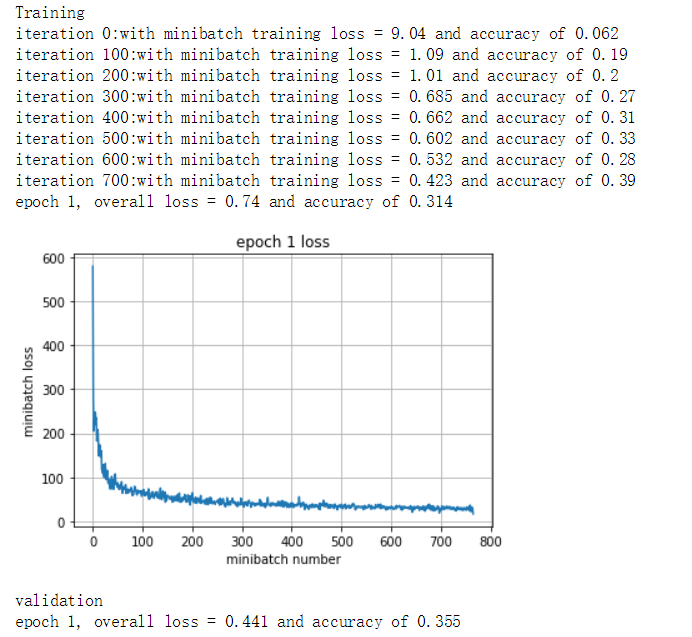
3、tensorflow搭建完整模型
内容参考:参考
由于加入了batchnorm(尤其注意),和pool所以代码要有一些改动。
from tensorflow.python.training import moving_averages
from tensorflow.python.ops import control_flow_ops

tf.reset_default_graph()

X = tf.placeholder(tf.float32,[None,32,32,3])
y = tf.placeholder(tf.int64,[None])
is_training = tf.placeholder(tf.bool)


def complex_model(X,y,is_traing):
    MOVING_AVERAGE_DECAY = 0.9997
    BN_DECAY = MOVING_AVERAGE_DECAY
    BN_EPSILON = 0.001

    Wconv1 = tf.get_variable('Wconv1',shape=[7,7,3,32])
    bconv1 = tf.get_variable('bconv1',shape=32)

    h1 = tf.nn.conv2d(X,Wconv1,strides=[1,1,1,1],padding='VALID') + bconv1
    a1 = tf.nn.relu(h1)   #a1.size = [batch_size,26,26,32]


    axis = list(range(len(a1.get_shape())-1))  #axis = [0,1,2]
    mean, variance = tf.nn.moments(a1,axis)    #求均值和方差,对特征的每一片求均值和方差

    params_shape = a1.get_shape()[-1:]   #取出通道数

    #每一篇卷积结果(feature map)都有一个beta和gamma
    beta = tf.get_variable('beta',params_shape,initializer=tf.zeros_initializer)
    gamma = tf.get_variable('gamma',params_shape,initializer=tf.ones_initializer)

    #移动平均值和移动方差在预测阶段使用
    moving_mean = tf.get_variable('moving_mean',params_shape,initializer=tf.zeros_initializer,trainable=False)
    moving_variance = tf.get_variable('moving_variance',params_shape,initializer=tf.ones_initializer,trainable=False)


    #更新移动平均值和移动方差
    update_moving_mean = moving_averages.assign_moving_average(moving_mean,mean,BN_DECAY)
    update_moving_variance = moving_averages.assign_moving_average(moving_variance,variance,BN_DECAY)
    tf.add_to_collection(tf.GraphKeys.UPDATE_OPS,update_moving_mean)
    tf.add_to_collection(tf.GraphKeys.UPDATE_OPS,update_moving_variance)

    mean, variance = control_flow_ops.cond(is_training,lambda:(mean,variance),lambda:(moving_mean,moving_variance))


    a1_b = tf.nn.batch_normalization(a1,mean,variance,beta,gamma,BN_EPSILON)

    #2x2的池化层,步长为2
    m1 = tf.nn.max_pool(a1_b,ksize=[1,2,2,1],strides=[1,2,2,1],padding='VALID')

    m1_flat = tf.reshape(m1, [-1,5408])
    W1 = tf.get_variable('W1',shape=[5408,1024])
    b1 = tf.get_variable('b1',shape=[1024])
    h2 = tf.matmul(m1_flat,W1)+b1

    a2=tf.nn.relu(h2)

    W2 = tf.get_variable('W2',shape=[1024,10])
    b2 = tf.get_variable('b2',shape=[10])
    y_out = tf.matmul(a2,W2)+b2
    return y_out

y_out = complex_model(X,y,is_traing)
4、模块化的卷积神经网络
模块化过程中和之前有所不一样:
1、tf.layers.conv2d(),参数被简化了许多,直接包含激活
2、tf.layers.max_pooling2d()
3、tf.layers.dense(),全连接网络部分
def my_model(X,y,is_training):
    def conv_relu_pool(X,num_filter=32,conv_strides=1,kernel_size=[3,3],pool_size=[2,2],pool_stride=2):
        conv1=tf.layers.conv2d(inputs=X,filters=num_filter,kernel_size=kernel_size,strides=conv_strides,padding='same',activation=tf.nn.relu)
        pool1 = tf.layers.max_pooling2d(inputs=conv1,pool_size=pool_size,strides=pool_stride)
        return pool1

    def conv_relu_conv_relu_pool(X,num_filter1 = 32,num_filter2=32,conv_strides=1,kernel_size=[5,5],pool_size=[2,2],pool_stride=2):
        conv1 = tf.layers.conv2d(inputs=X,filters=num_filter1,kernel_size=kernel_size,strides=conv_strides,padding='same',activation=tf.nn.relu)
        conv2 = tf.layers.conv2d(inputs=conv1,filters=num_filter2,kernel_size=kernel_size,strides=conv_strides,padding='same',activation=tf.nn.relu)
        pool1 = tf.layers.max_pooling2d(inputs=conv2,pool_size=pool_size,strides=pool_stride)
        return pool1

    def affline(X, num_units, act):
        #全连接层
        return tf.layers.dense(inputs=X, units=num_units,activation=act)

    def batchnorm_relu_conv(X, num_filters =32, conv_strides=2,kernel_size=[5,5],is_training=True):
        bat1 = tf.layers.batch_normalization(X,training=is_training)
        act1 = tf.nn.relu(bat1)
        conv1 = tf.layers.conv2d(inputs=act1,filters=num_filters,kernel_size=kernel_size,strides=2,padding='same',activation=None)
        return conv1

    N = 3 #num of conv blocks
    M = 1 #num of affine
    #因为需要batchnorm,所以不激活
    conv = tf.layers.conv2d(inputs=X,filters=64,kernel_size=[5,5],strides=1,padding='same',activation=None)

    for i in range(N):
        print(conv.get_shape())
        conv = batchnorm_relu_conv(conv,is_training=is_training)

    print(conv.get_shape())
    global_average_shape = conv.get_shape()[1:3]

    avg_layer = tf.reduce_mean(conv,[1,2])
    print(avg_layer.get_shape())

    fc = avg_layer
    for i in range(M):
        fc = affline(fc,100,tf.nn.relu)

    fc = affline(fc,10,None)
    return fc

tf.reset_default_graph()
X = tf.placeholder(tf.float32,[None,32,32,3])
y = tf.placeholder(tf.int64,[None])
is_training = tf.placeholder(tf.bool)

y_out = my_model(X,y,is_training)
total_loss = tf.nn.softmax_cross_entropy_with_logits(logits=y_out,labels=tf.one_hot(y,10))
mean_loss = tf.reduce_mean(total_loss)


#batch-norm需要的代码
global_step = tf.Variable(0,trainable=False,name="Global_Step")
starter_learning_rate = 1e-2
#学习率的下降
learning_rate = tf.train.exponential_decay(starter_learning_rate,global_step,750,0.96,staircase=True)

optimizer = tf.train.AdamOptimizer(learning_rate)

extra_update_ops = tf.get_collection(tf.GraphKeys.UPDATE_OPS)
with tf.control_dependencies(extra_update_ops):
    train_step = optimizer.minimize(mean_loss,global_step = global_step)

print([x.name for x in tf.global_variables()])

sess = tf.Session()
sess.run(tf.global_variables_initializer())
print('Training')
run_model(sess,y_out,mean_loss,X_train,y_train,2,64,100,train_step,True)
print('Vaildation')
run_model(sess,y_out,mean_loss,X_val,y_val,1,64)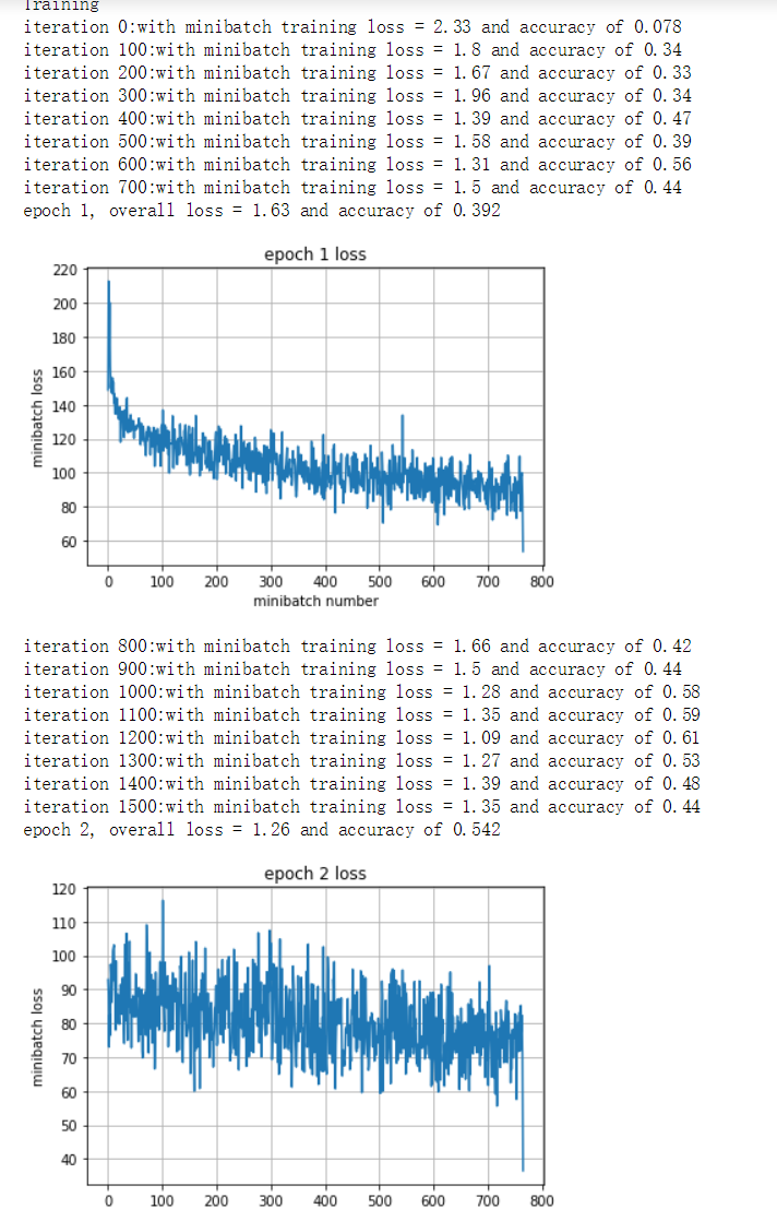
最后
以上就是飘逸小猫咪最近收集整理的关于cs231n assignment(二) Tensorflow以及卷积神经网络序1、读取cifar10图像2、tensorflow搭建简单模型3、tensorflow搭建完整模型4、模块化的卷积神经网络的全部内容,更多相关cs231n内容请搜索靠谱客的其他文章。


发表评论 取消回复