R QQplot的demo和理解

101 阅读 0 评论 67 点赞

我是靠谱客的博主追寻大门，这篇文章主要介绍R QQplot的demo和理解，现在分享给大家，希望可以做个参考。

R QQplot的demo和理解

- 需要的library
- 正态分布样例 (Samples for ????(0,1))
- 右偏分布样例 (Samples for right skewed distribution）
- 左偏分布样例(Samples for left skewed distribution)
- 短尾分布样例 (Samples for shot tailed distribution)
- 总结
- 写在最后

需要的library

复制代码

1
2
3
library("car")
library(fGarch)

正态分布样例 (Samples for ????(0,1))

复制代码

1
2
3
4
5
6
7
8
9
set.seed(0)
x <- rnorm(1000, mean = 0, sd = 1)
par(mfrow = c(1, 2), pty = "s")
qqPlot(x, main="QQ Plot")
hist(x, n = 50, freq=FALSE, main="Distribution of Residuals", border = "white", col = "steelblue")
#xfit<-seq(min(x),max(x),length=50) 
#yfit<-dnorm(xfit) 
#lines(xfit, yfit, col = 'red', lwd = 3)

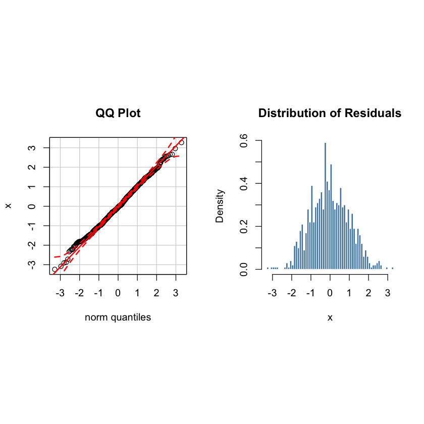正态分布qqplot 可以看到上图qqplot图（左图）的点基本都躺在红色拟合线上，这种图像表明数据分布是近似正态分布。
右图为同数据生成的分布图，下同。

右偏分布样例 (Samples for right skewed distribution）

复制代码

1
2
3
4
5
6
7
8
9
10
set.seed(0)
par(mfrow = c(1, 2), pty = "s")
snorm = rsnorm(1000, mean = 0, sd = 1, xi = 3)
qqPlot(snorm, main="QQ Plot")
#hist(snorm, Probability=True, main="Distribution of Residuals")
hist(snorm, n = 25, probability = TRUE, border = "white", col = "steelblue")
#xfit<-seq(min(snorm),max(snorm),length=50) 
#yfit<-dnorm(xfit) 
#lines(xfit, yfit, col = 'red', lwd = 3)

右偏分布qqplot
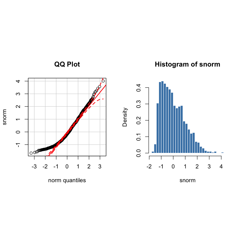
上图qqplot图红色拟合线的起点和终点都位于对角线（y=x）下方，或者说右方，则这种qqplot图像表示数据分布为右偏分布。

左偏分布样例(Samples for left skewed distribution)

复制代码

1
2
3
4
5
6
7
8
9
set.seed(0)
par(mfrow = c(1, 2), pty = "s")
snorm = rsnorm(1000, mean = 0, sd = 1, xi = -3)
qqPlot(snorm, main="QQ Plot")
hist(snorm, n=50, freq=FALSE, main="Distribution of Residuals",  border = "white", col = "steelblue")
#xfit<-seq(min(snorm),max(snorm),length=50) 
#yfit<-dnorm(xfit) 
#lines(xfit, yfit, col = 'red', lwd = 3)

左偏分布qqplot
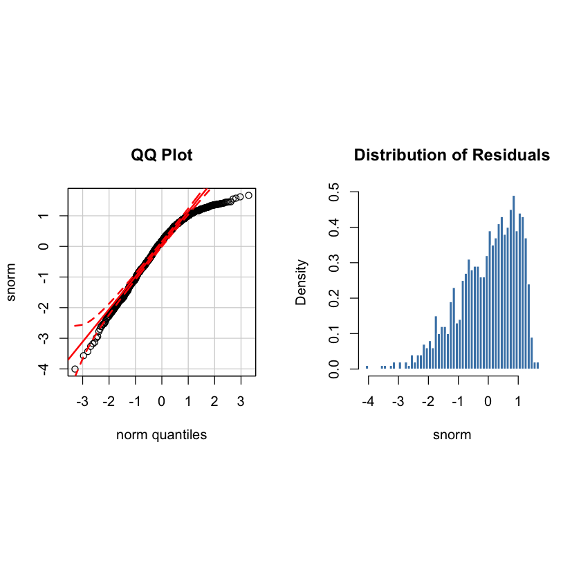
上图qqplot图红色拟合线的起点和终点都位于对角线（y=x）上方，或者说左方，则这种qqplot图像表示数据分布为左偏分布。

短尾分布样例 (Samples for shot tailed distribution)

复制代码

1
2
3
4
5
6
set.seed(0)
par(mfrow = c(1, 2), pty = "s")
short = runif(1000,min=0,max=2)
qqPlot(short, main="QQ Plot")
hist(short, n=100, freq=FALSE, main="Distribution of Residuals",  border = "white", col = "steelblue")

短尾分布1

复制代码

1
2
3
4
5
6
7
8
9
set.seed(0)
par(mfrow = c(1, 2), pty = "s")
long <- rcauchy(1000, location = 0, scale=1)
qqPlot(long, main="QQ Plot")
hist(long, n=100, freq=FALSE, main="Distribution of Residuals",  border = "white", col = "steelblue")
#xfit<-seq(min(long),max(long),length=100) 
#yfit<-dcauchy(xfit) 
#lines(xfit, yfit, col = 'red', lwd = 3)

短尾分布2
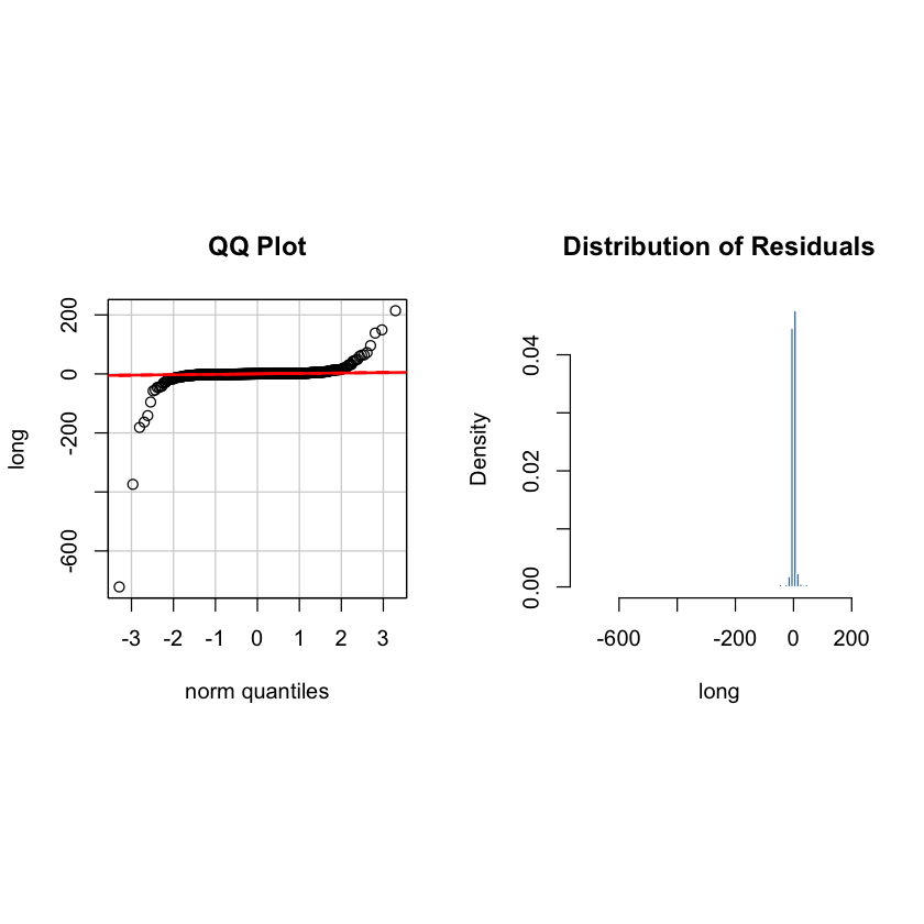
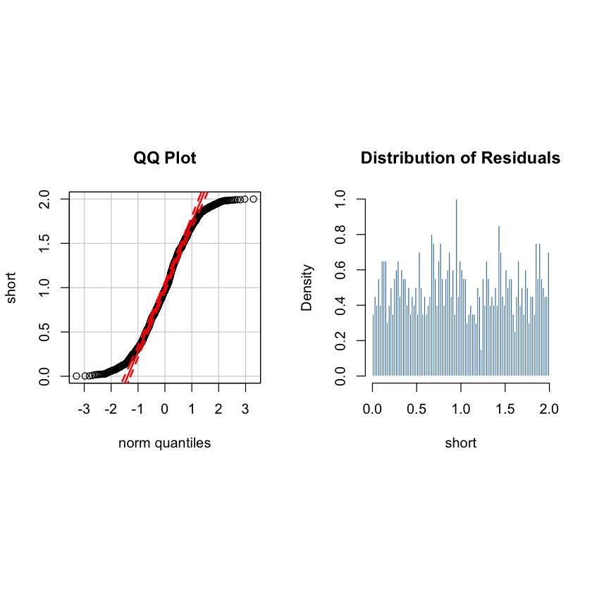
由以上2个样例可以看出，当qqplot图的拟合线与对角线（y=x）有交叉时，且该拟合线比较接近水平或竖直时，则这种qqplot图像表明数据是分布是短尾分布。

总结

qqplot 是一种较为便捷的方法来判断数据分布是怎么样的。
那么就会有人问，直接拿hist()看分布不香吗？
我是同意上面这种想法的。
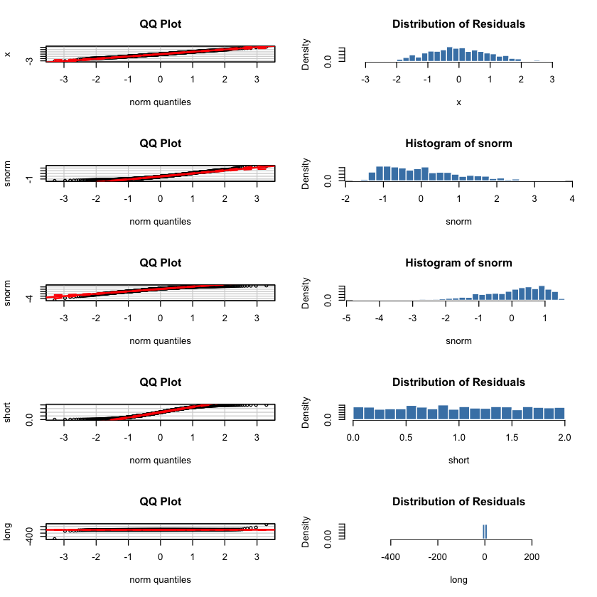
我理解qqplot核心是用来比较两组数据分布是否类似。
什么意思？
将上面的例子换个方式思考，你就会明白。
前面举的例子都是用我们创造的一组数据跟正态分布的数据进行比较。
换句话说，就是我们创造的这组数据的分布跟正态分布数据的分布是不是一样的。
如果把正态分布的数据换成其他的数据，不就成了比较A，B两组数据的分布是否是一样的了嘛~

复制代码

1
2
3
4
5
6
7
8
9
10
11
12
13
14
15
16
17
18
19
20
21
22
23
par(mfrow = c(5, 2))
set.seed(0)

x <- rnorm(1000, mean = 0, sd = 1)
qqPlot(x, main="QQ Plot")
hist(x, n = 25, freq=FALSE, main="Distribution of Residuals", border = "white", col = "steelblue")

snorm = rsnorm(1000, mean = 0, sd = 1, xi = 3)
qqPlot(snorm, main="QQ Plot")
hist(snorm, n = 25, probability = TRUE, border = "white", col = "steelblue")

snorm = rsnorm(1000, mean = 0, sd = 1, xi = -3)
qqPlot(snorm, main="QQ Plot")
hist(snorm, n = 25, probability = TRUE, border = "white", col = "steelblue")

short = runif(1000,min=0,max=2)
qqPlot(short, main="QQ Plot")
hist(short, n=25, freq=FALSE, main="Distribution of Residuals",  border = "white", col = "steelblue")

long <- rcauchy(1000, location = 0, scale=0.5)
qqPlot(long, main="QQ Plot")
hist(long, n=100, freq=FALSE, main="Distribution of Residuals",  border = "white", col = "steelblue")