目录
0. 前言
1. 算法原理
2. Python仿真
2.1 函数改造
2.2 softmax()
2.3 改造后的k_armed_bandit_one_run()
2.4 对比仿真
2.5 一点异常
3. 练习题
4. 小结
0. 前言
前面几节我们已经就多臂老虎机问题进行了一些讨论。详细参见本系列总目录:
强化学习笔记总目录 https://blog.csdn.net/chenxy_bwave/article/details/121715424
本节我们继续基于多臂老虎机问题学习一种基于梯度下降的行动选择方法:Gradient Bandit Algorithm
Ref: Sutton-RLBook2020-2.8: Gradient Bandit Algotihm
1. 算法原理
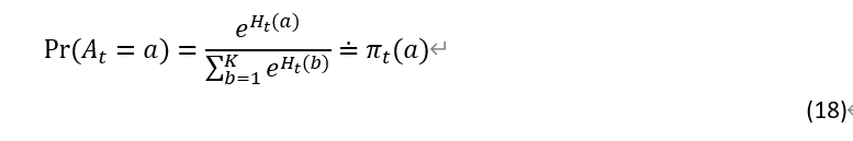
前面所考虑得都是估计行动价值(action values)然后基于这些估计值进行行动选择。通常来说这是一个好得方法,但是并非唯一可能的方法。本节我们考虑另一种方法,对每个行动估计一个数值优先度(numeric preference)度量值,记为![]() . 这个优先度量表示我们应该选择该行动的概率(该优先度量越大,则选择该行动的概率越高)。但是这个优先度量并不反映奖励的绝对量,重要的只是各行动之间的相关优先度,比如说,给所有各行动的优先度量都加上1000,这个并不改变它们被选择的概率。从优先度量
. 这个优先度量表示我们应该选择该行动的概率(该优先度量越大,则选择该行动的概率越高)。但是这个优先度量并不反映奖励的绝对量,重要的只是各行动之间的相关优先度,比如说,给所有各行动的优先度量都加上1000,这个并不改变它们被选择的概率。从优先度量![]() 到行动概率的映射由soft-max distribution(i.e., Gibbs or Boltzmann distribution)决定:
到行动概率的映射由soft-max distribution(i.e., Gibbs or Boltzmann distribution)决定:
以上我们引入了一个新符号![]() 用于表示选择行动的概率,这可以理解为一种策略(policy)。顺便说一句,在强化学习中,通常用π
用于表示选择行动的概率,这可以理解为一种策略(policy)。顺便说一句,在强化学习中,通常用π![]() 表示策略(policy)。所有行动的优先度量都初始化为0,意味着在一开始它们被选择的概率相等。
表示策略(policy)。所有行动的优先度量都初始化为0,意味着在一开始它们被选择的概率相等。
对于以上这个基于soft-max分布的行动概率策略有一个很自然的学习算法,那就是随机梯度下降算法(SGD: stochastic gradient ascent),在每一步采取行动At 然后收到奖励Rt, 行动优先度量按如下方式更新:
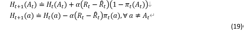
![]() 表示步长参数,
表示步长参数,![]() 表示到t时刻(不包含时刻t)之前的奖励平均值(
表示到t时刻(不包含时刻t)之前的奖励平均值(![]() ),可以以前面介绍过的递增式的方式计算(section 2.4, or 2.5 if the problem is nonstationary)。其物理意义很直观,
),可以以前面介绍过的递增式的方式计算(section 2.4, or 2.5 if the problem is nonstationary)。其物理意义很直观,![]() 代表当前At得到的奖励Rt,如果比之前得到的奖励的平均值大,就提高它的优先度量,即在后续行动中选择它的概率进一步提高,反之亦然;其它行动的概率变化总是与At的相反(因为总概率为1)。
代表当前At得到的奖励Rt,如果比之前得到的奖励的平均值大,就提高它的优先度量,即在后续行动中选择它的概率进一步提高,反之亦然;其它行动的概率变化总是与At的相反(因为总概率为1)。
2. Python仿真
2.1 函数改造
基于上一篇中的k_armed_bandit_one_run()进行改造。
(1) 追加一个函数softmax()--应该能比如说scikit-learn等库中找到,不过嘛,自己写一个也是一个练习
(2) 追加参数actsel='SGD'的选项
(3) 在actsel设定为'SGD'时,调用softmax()以更新各行动的H(preference)值
(4) 追加baseline参数用于当actsel=SGD时,选择有baseline还是没有baseline
2.2 softmax()
softmax()函数如下所示:
def softmax(H):
    """
    Input:
        H: Preference input
    Output:
        P: Probability
    """
    L = len(H)
    H_exp = np.exp(H)
    P = H_exp / np.sum(H_exp)

    if not np.isclose(np.sum(P), 1): # The sum of probability should be one.
        print('softmax(): error!')

    return P
2.3 改造后的k_armed_bandit_one_run()
改造后的k_armed_bandit_one_run() 如下所示:
def k_armed_bandit_one_run(qstar,epsilon,nStep,Qinit,QUpdtAlgo='sample_average',alpha=0, stationary=True, actsel=None, baseline=True):
    """
    One run of K-armed bandit simulation.
    Add Qinit to the interface.
    Input:
        qstar:     Mean reward for each candition actions
        epsilon:   Epsilon value for epsilon-greedy algorithm
        nStep:     The number of steps for simulation
        Qinit:     Initial setting for action-value estimate
        QUpdtAlgo: The algorithm for updating Q value--'sample_average','exp_decaying'
        alpha:     step-size in case of 'exp_decaying' and also used in case of actsel='SGD'
        actsel:    Specifying action selection algorithm
        baseline:  'Yes','No' for actsel=SGD
    Output:
        a[t]: action series for each step in one run
        r[t]: reward series for each step in one run
        Q[k]: reward sample average up to t-1 for action[k]
        aNum[k]: The number of being selected for action[k]
        optRatio[t]: Ration of optimal action being selected over tim
    """
    K     = len(qstar)
    Q     = Qinit
    a     = np.zeros(nStep+1,dtype='int') # Item#0 for initialization
    aNum  = np.zeros(K,dtype='int')       # Record the number of action#k being selected

    H     = np.zeros(K,dtype='int')       # Record the preference of all actions, and initialized to all zeros, for Gradient algorithm
    P     = softmax(H)
    r     = np.zeros(nStep+1)             # Record the award received at each time step. r[0] for initialization

    average_reward = 0                    # Used for SGD action selection algorithm. Note the difference bwteen this and Q!

    if stationary == False:
        qstar = np.ones(K)/K              # qstart initialized to 1/K for all K actions

    optCnt   = 0
    optRatio = np.zeros(nStep+1,dtype='float') # Item#0 for initialization

    for t in range(1,nStep+1):

        #0. For non-stationary environment, optAct also changes over time.Hence, move to inside the loop.
        optAct   = np.argmax(qstar)

        #1. action selection
        if actsel == 'UCB':
            aMax = -np.Inf
            for k in range(K):
                if aNum[k] == 0:
                    aMetric = np.inf
                else:
                    aMetric = Q[k] + epsilon * np.sqrt(np.log(t)/aNum[k])
                if aMax < aMetric:
                    aOpt = k
                    aMax = aMetric
            a[t] = aOpt
        elif actsel == 'SGD':
            # Calculate the probability of all actions based on the H preference
            P     = softmax(H)
            # Choose the action based on the probability
            a[t] = np.random.choice([k for k in range(K)], size=1,replace=True, p=P)
        else:
            tmp = np.random.uniform(0,1)
            if tmp < epsilon: # random selection
                a[t] = np.random.choice(np.arange(K))
                #print('random selection: a[{0}] = {1}'.format(t,a[t]))
            else:             # greedy selection
                #选择Q值最大的那个,当多个Q值并列第一时,从中任选一个--但是如何判断有多个并列第一的呢?
                #对Q进行random permutation处理后再找最大值可以等价地解决这个问题
                p = np.random.permutation(K)
                a[t] = p[np.argmax(Q[p])]
                #print('greedy selection: a[{0}] = {1}'.format(t,a[t]))

        aNum[a[t]] = aNum[a[t]] + 1

        #2. reward: draw from the pre-defined probability distribution
        r[t] = np.random.randn() + qstar[a[t]]

        #3.Update Q of the selected action - #2.4 Incremental Implementation
        # Q[a[t]] = (Q[a[t]]*(aNum[a[t]]-1) + r[t])/aNum[a[t]]
        if QUpdtAlgo == 'sample_average':
            Q[a[t]] = Q[a[t]] + (r[t]-Q[a[t]])/aNum[a[t]]
        elif QUpdtAlgo == 'exp_decaying':
            Q[a[t]] = Q[a[t]] + (r[t]-Q[a[t]])*alpha

        #4. Optimal Action Ratio tracking
        #print(a[t], optAct)
        if a[t] == optAct:
            optCnt = optCnt + 1
        optRatio[t] = optCnt/t

        #5. Random walk of qstar simulating non-stationary environment
        # Take independent random walks (say by adding a normally distributed increment with mean 0
        # and standard deviation 0.01 to all the q*(a) on each step).
        if stationary == False:
            qstar = qstar + np.random.randn(K)*0.01 # Standard Deviation = 0.01
            #print('t={0}, qstar={1}, sum={2}'.format(t,qstar,np.sum(qstar)))

        #6. Update H preference
        H_At_old = H[a[t]] # backoff for later use
        H = H - alpha*(r[t]-average_reward)*P
        H[a[t]] = H_At_old + alpha*(r[t]-average_reward)*(1-P[a[t]])

        #7. Update average_reward
        if baseline:
            #average_reward += (r[t] - average_reward)/t
            average_reward = np.mean(r[1:]) # NG, but why?

    return a,aNum,r,Q,optRatio
2.4 对比仿真
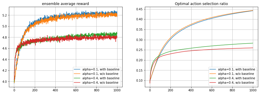
针对以下4种情况进行对比仿真:
SGD, stationary environment,
(1) alpha = 0.1, with baseline
(2) alpha = 0.1, without baseline
(3) alpha = 0.4, with baseline
(4) alpha = 0.4, without baseline
import numpy as np
import matplotlib.pyplot as plt
%matplotlib inline

nStep = 1000
nRun  = 2000
K     = 10

r_1   = np.zeros((nRun,nStep+1))
r_2   = np.zeros((nRun,nStep+1))
r_3   = np.zeros((nRun,nStep+1))
r_4   = np.zeros((nRun,nStep+1))
optRatio_1 = np.zeros((nRun,nStep+1))
optRatio_2 = np.zeros((nRun,nStep+1))
optRatio_3 = np.zeros((nRun,nStep+1))
optRatio_4 = np.zeros((nRun,nStep+1))

Qinit = np.zeros(K)
epsilon = 0

for run in range(nRun):
    print('.',end='')
    if run%100==99:
        print('run = ',run+1)

    qstar   = np.random.randn(10) + 4
    a,aNum,r_1[run,:],Q,optRatio_1[run,:] = k_armed_bandit_one_run(qstar,epsilon,nStep,Qinit, alpha=0.1,actsel='SGD',baseline=True)
    a,aNum,r_2[run,:],Q,optRatio_2[run,:] = k_armed_bandit_one_run(qstar,epsilon,nStep,Qinit, alpha=0.1,actsel='SGD',baseline=False)
    a,aNum,r_3[run,:],Q,optRatio_3[run,:] = k_armed_bandit_one_run(qstar,epsilon,nStep,Qinit, alpha=0.4,actsel='SGD',baseline=True)
    a,aNum,r_4[run,:],Q,optRatio_4[run,:] = k_armed_bandit_one_run(qstar,epsilon,nStep,Qinit, alpha=0.4,actsel='SGD',baseline=False)
# Plotting
rEnsembleMean_1 = np.mean(r_1,axis=0)
rEnsembleMean_2 = np.mean(r_2,axis=0)
rEnsembleMean_3 = np.mean(r_3,axis=0)
rEnsembleMean_4 = np.mean(r_4,axis=0)
optRatioEnsembleMean_1 = np.mean(optRatio_1,axis=0)
optRatioEnsembleMean_2 = np.mean(optRatio_2,axis=0)
optRatioEnsembleMean_3 = np.mean(optRatio_3,axis=0)
optRatioEnsembleMean_4 = np.mean(optRatio_4,axis=0)
fig,ax = plt.subplots(1,2,figsize=(15,5))
ax[0].plot(rEnsembleMean_1[1:]) # Note: t count from 1 in k_armed_bandit_one_run()
ax[0].plot(rEnsembleMean_2[1:])
ax[0].plot(rEnsembleMean_3[1:])
ax[0].plot(rEnsembleMean_4[1:])
ax[0].legend(['alpha=0.1, with baseline','alpha=0.1, w/o baseline','alpha=0.4, with baseline','alpha=0.4, w/o baseline'])
ax[0].set_title('ensemble average reward')
ax[0].grid()
ax[1].plot(optRatioEnsembleMean_1[1:])
ax[1].plot(optRatioEnsembleMean_2[1:])
ax[1].plot(optRatioEnsembleMean_3[1:])
ax[1].plot(optRatioEnsembleMean_4[1:])
ax[1].legend(['alpha=0.1, with baseline','alpha=0.1, w/o baseline','alpha=0.4, with baseline','alpha=0.4, w/o baseline'])
ax[1].set_title('Optimal action selection ratio')
ax[1].grid()得到结果如下:
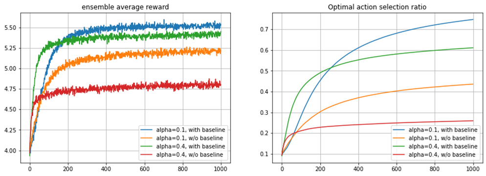
右图与书中的Figure2.5略有差异。 但是总体上来说是吻合。因为是2000次运行的总体平均,按道理来说是应该要更加一致才合理。估计在实现细节上与输出原书的图的实现代码还是有细微差异。
2.5 一点异常
在以上仿真试验中发现一个小小的异常现象,average_reward的计算方法的一个小小微调对结果产生相当显著的影响:
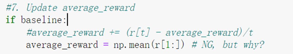
 对比以上两个图,可知,总体平均奖励和最优行动选择比率都大幅度恶化了。原因不明,有待进一步学习研究。
3. 练习题
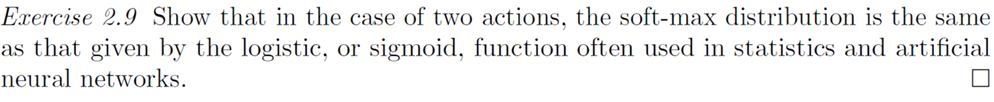
Solution:
考虑两个action: a1, a2. 对应的H-preference分别为H1,H2, 则根据soft-max distribution,可得:
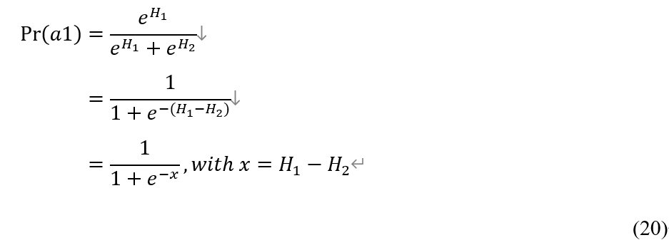
式(20)恰是sigmoid函数的表现形式。
4. 小结
以上我们结合仿真学习了Gradient Bandit Algorithm。有一个遗留问题就是算法行为似乎对average_reward计算方法非常敏感,在增加步长后这种敏感性会慢慢消失吗?
另外,原书中给出关于Gradient Bandit Algorithm的公式的理论推导,这里就不再搬运了。有兴趣的兴趣(当然光有兴趣还不够,还需要一丢丢数学功底^-^)可以找原书自行学习。
最后
以上就是温暖糖豆最近收集整理的关于强化学习笔记:多臂老虎机问题(7)--Gradient Bandit Algorithm0. 前言1. 算法原理2. Python仿真3. 练习题4. 小结的全部内容,更多相关强化学习笔记:多臂老虎机问题(7)--Gradient内容请搜索靠谱客的其他文章。


发表评论 取消回复