目录
- 1 引言
- 2 Python实现
- 2.1 初始化和定义函数
- 2.1.1 初始化参数
- 2.1.2 可视化导频插入的格式
- 2.1.3 定义调制和解调方式
- 2.1.4 定义信道
- 2.2 OFDM仿真过程
- 2.2.1 发送端
- 2.2.2 信道
- 2.2.3 接收端
1 引言
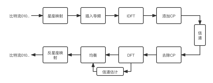
OFDM的通信系统仿真,Matlab实现的版本比比皆是,Python版本的底层详细的仿真过程缺少之又少,本人根据Commpy工具包,实现了OFDM的信号发射、经过信道、接收端接收的过程。实现的调制方式有BPSK、QPSK、8PSK、16QAM、64QAM。并可视化了导频的插入方式、信道冲击响应、信号解调前的星座映射和解调后的星座映射,以及计算了仿真系统的误比特率。完整代码的见本人的githubPython实现OFDM仿真
commpy包的官方文档https://commpy.readthedocs.io/en/latest/index.html
commpy包的安装方式
pip install scikit-commpy
2 Python实现
2.1 初始化和定义函数
2.1.1 初始化参数
导入包
import numpy as np
import matplotlib.pyplot as plt
from scipy import interpolate
import commpy as cpy
K = 64 # OFDM子载波数量
CP = K//4  #25%的循环前缀长度
P = 8  # 导频数
pilotValue = 3+3j  # 导频格式
Modulation_type = 'QAM16' #调制方式,可选BPSK、QPSK、8PSK、QAM16、QAM64
channel_type ='random' # 信道类型,可选awgn
SNRdb = 25  # 接收端的信噪比(dB)
allCarriers = np.arange(K)  # 子载波编号 ([0, 1, ... K-1])
pilotCarrier = allCarriers[::K//P]  # 每间隔P个子载波一个导频
# 为了方便信道估计,将最后一个子载波也作为导频
pilotCarriers = np.hstack([pilotCarrier, np.array([allCarriers[-1]])])
P = P+1 # 导频的数量也需要加1
2.1.2 可视化导频插入的格式
# 可视化数据和导频的插入方式
dataCarriers = np.delete(allCarriers, pilotCarriers)
plt.figure(figsize=(8, 0.8))
plt.plot(pilotCarriers, np.zeros_like(pilotCarriers), 'bo', label='pilot')
plt.plot(dataCarriers, np.zeros_like(dataCarriers), 'ro', label='data')
plt.legend(fontsize=10, ncol=2)
plt.xlim((-1, K))
plt.ylim((-0.1, 0.3))
plt.xlabel('Carrier index')
plt.yticks([])
plt.grid(True)
plt.savefig('carrier.png')

2.1.3 定义调制和解调方式
m_map = {"BPSK": 1, "QPSK": 2, "8PSK": 3, "QAM16": 4, "QAM64": 6}
mu = m_map[Modulation_type]
payloadBits_per_OFDM = len(dataCarriers)*mu  # 每个 OFDM 符号的有效载荷位数
# 定制调制方式
def Modulation(bits):
    if Modulation_type == "QPSK":
        PSK4 = cpy.PSKModem(4)
        symbol = PSK4.modulate(bits)
        return symbol
    elif Modulation_type == "QAM64":
        QAM64 = cpy.QAMModem(64)
        symbol = QAM64.modulate(bits)
        return symbol
    elif Modulation_type == "QAM16":
        QAM16 = cpy.QAMModem(16)
        symbol = QAM16.modulate(bits)
        return symbol
    elif Modulation_type == "8PSK":
        PSK8 = cpy.PSKModem(8)
        symbol = PSK8.modulate(bits)
        return symbol
    elif Modulation_type == "BPSK":
        BPSK = cpy.PSKModem(2)
        symbol = BPSK.modulate(bits)
        return symbol
# 定义解调方式
def DeModulation(symbol):
    if Modulation_type == "QPSK":
        PSK4 = cpy.PSKModem(4)
        bits = PSK4.demodulate(symbol, demod_type='hard')
        return bits
    elif Modulation_type == "QAM64":
        QAM64 = cpy.QAMModem(64)
        bits = QAM64.demodulate(symbol, demod_type='hard')
        return bits
    elif Modulation_type == "QAM16":
        QAM16 = cpy.QAMModem(16)
        bits = QAM16.demodulate(symbol, demod_type='hard')
        return bits
    elif Modulation_type == "8PSK":
        PSK8 = cpy.PSKModem(8)
        bits = PSK8.demodulate(symbol, demod_type='hard')
        return bits
    elif Modulation_type == "BPSK":
        BPSK = cpy.PSKModem(2)
        bits = BPSK.demodulate(symbol, demod_type='hard')
        return bits
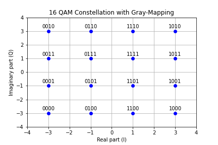
调制方式就是将比特流映射到星座图,得到了复数数值,在信道中以复数数值进行传输。
16QAM的星座图,如下图所示
2.1.4 定义信道
# 可视化信道冲击响应,仿真信道
# the impulse response of the wireless channel
channelResponse = np.array([1, 0, 0.3+0.3j])
H_exact = np.fft.fft(channelResponse, K)
plt.plot(allCarriers, abs(H_exact))
plt.xlabel('Subcarrier index')
plt.ylabel('$|H(f)|$')
plt.grid(True)
plt.xlim(0, K-1)
# 定义信道
def add_awgn(x_s, snrDB):
    data_pwr = np.mean(abs(x_s**2))
    noise_pwr = data_pwr/(10**(snrDB/10))
    noise = 1/np.sqrt(2) * (np.random.randn(len(x_s)) + 1j *
                            np.random.randn(len(x_s))) * np.sqrt(noise_pwr)
    return x_s + noise, noise_pwr
def channel(in_signal, SNRdb, channel_type="awgn"):
    channelResponse = np.array([1, 0, 0.3+0.3j]) #随意仿真信道冲击响应
    if channel_type == "random":
        convolved = np.convolve(in_signal, channelResponse)
        out_signal, noise_pwr = add_awgn(convolved, SNRdb)
    elif channel_type == "awgn":
        out_signal, noise_pwr = add_awgn(in_signal, SNRdb)
    return out_signal, noise_pwr
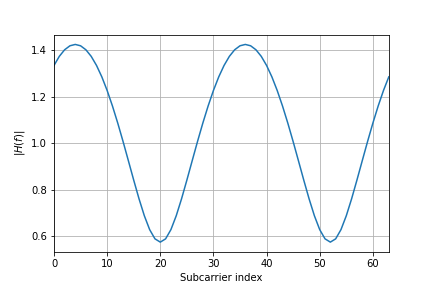
可视化冲击响应图,此处的信道衰落,只是举例实现了简单的一个冲击响应波形。复杂的信道模型,根据自己的信道去实现仿真过程。awgn表示加入高斯噪声。
2.2 OFDM仿真过程
2.2.1 发送端
# 5.1 产生比特流
bits = np.random.binomial(n=1, p=0.5, size=(payloadBits_per_OFDM, ))
# 5.2 比特信号调制
QAM_s = Modulation(bits)
# 5.3 插入导频和数据,生成OFDM符号
def OFDM_symbol(QAM_payload):
    symbol = np.zeros(K, dtype=complex) # 子载波位置
    symbol[pilotCarriers] = pilotValue  # 在导频位置插入导频
    symbol[dataCarriers] = QAM_payload  # 在数据位置插入数据
    return symbol
OFDM_data = OFDM_symbol(QAM_s)
# 5.4 快速傅里叶逆变换
def IDFT(OFDM_data):
    return np.fft.ifft(OFDM_data)
OFDM_time = IDFT(OFDM_data)
# 5.5 添加循环前缀
def addCP(OFDM_time):
    cp = OFDM_time[-CP:]
    return np.hstack([cp, OFDM_time])
OFDM_withCP = addCP(OFDM_time)
2.2.2 信道
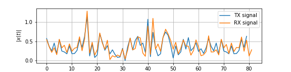
经过信道,可视化加入冲击响应后的信号和原始信号的波形
# 5.6 经过信道
OFDM_TX = OFDM_withCP
OFDM_RX = channel(OFDM_TX, SNRdb, "random")[0]
plt.figure(figsize=(8,2))
plt.plot(abs(OFDM_TX), label='TX signal')
plt.plot(abs(OFDM_RX), label='RX signal')
plt.legend(fontsize=10)
plt.xlabel('Time'); plt.ylabel('$|x(t)|$');
plt.grid(True);
# plt.savefig('tran-receiver.png')
2.2.3 接收端
接收端,首先去循环前缀、再快速傅里叶变换、再进行信道估计,再以信道估计的冲击响应去均衡信号,
# 5.7 接收端,去除循环前缀
def removeCP(signal):
return signal[CP:(CP+K)]
OFDM_RX_noCP = removeCP(OFDM_RX)
# 5.8 快速傅里叶变换
def DFT(OFDM_RX):
return np.fft.fft(OFDM_RX)
OFDM_demod = DFT(OFDM_RX_noCP)
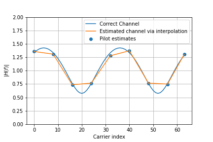
# 5.9 信道估计
def channelEstimate(OFDM_demod):
pilots = OFDM_demod[pilotCarriers] # 取导频处的数据
Hest_at_pilots = pilots / pilotValue # LS信道估计
# 在导频载波之间进行插值以获得估计,然后利用插值估计得到数据下标处的信道响应
Hest_abs = interpolate.interp1d(pilotCarriers, abs(Hest_at_pilots), kind='linear')(allCarriers)
Hest_phase = interpolate.interp1d(pilotCarriers, np.angle(Hest_at_pilots), kind='linear')(allCarriers)
Hest = Hest_abs * np.exp(1j*Hest_phase)
plt.plot(allCarriers, abs(H_exact), label='Correct Channel')
plt.scatter(pilotCarriers, abs(Hest_at_pilots), label='Pilot estimates')
plt.plot(allCarriers, abs(Hest), label='Estimated channel via interpolation')
plt.grid(True); plt.xlabel('Carrier index'); plt.ylabel('$|H(f)|$'); plt.legend(fontsize=10)
plt.ylim(0,2)
plt.savefig('信道响应估计.png')
return Hest
Hest = channelEstimate(OFDM_demod)
图中所示蓝色点表示信道估计点,黄色的连接线表示估计的冲击响应波形。
# 5.10 均衡
def equalize(OFDM_demod, Hest):
return OFDM_demod / Hest
equalized_Hest = equalize(OFDM_demod, Hest)
def get_payload(equalized):
return equalized[dataCarriers]
QAM_est = get_payload(equalized_Hest)
# 5.10 获取数据位置的数据
def get_payload(equalized):
return equalized[dataCarriers]
QAM_est = get_payload(equalized_Hest)
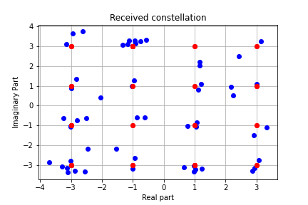
# 可视化均衡后的星座图
plt.plot(QAM_est.real, QAM_est.imag, 'bo')
plt.plot(QAM_s.real, QAM_s.imag, 'ro')
plt.grid(True)
plt.xlabel('Real part')
plt.ylabel('Imaginary Part')
plt.title("Received constellation")
plt.savefig('map.png')
# 5.11 反映射,解调
bits_est = DeModulation(QAM_est)
# 5.12 计算误比特率
print ("误比特率BER: ", np.sum(abs(bits-bits_est))/len(bits))
最后
以上就是贤惠水池最近收集整理的关于【Python】Python 仿真OFDM发射机、信道和接收机-实现多种调制方式1 引言2 Python实现的全部内容,更多相关【Python】Python内容请搜索靠谱客的其他文章。
本图文内容来源于网友提供,作为学习参考使用,或来自网络收集整理,版权属于原作者所有。


发表评论 取消回复