自动驾驶系列
车道曲率和中心点偏离距离计算
目标
知道车道曲率计算的方法
知道计算中心点偏离距离的计算
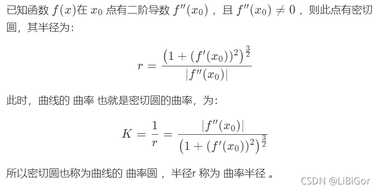
一、曲率的介绍
曲线的曲率就是针对曲线上某个点的切线方向角对弧长的转动率,通过微分来定义,表明曲线偏离直线的程度。数学上表明曲线在某一点的弯曲程度的数值。曲率越大,表示曲线的弯曲程度越大。曲率的倒数就是曲率半径。
圆的曲率
下面有三个球体,网球、篮球、地球,半径越小的越容易看出是圆的,所以随着半径的增加,圆的程度就越来越弱了。

定义球体或者圆的“圆”的程度,就是 曲率 ,计算方法为:
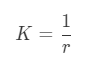
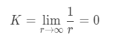
其中rr为球体或者圆的半径,这样半径越小的圆曲率越大,直线可以看作半径为无穷大的圆,其曲率为:
曲线的曲率
不同的曲线有不同的弯曲程度:
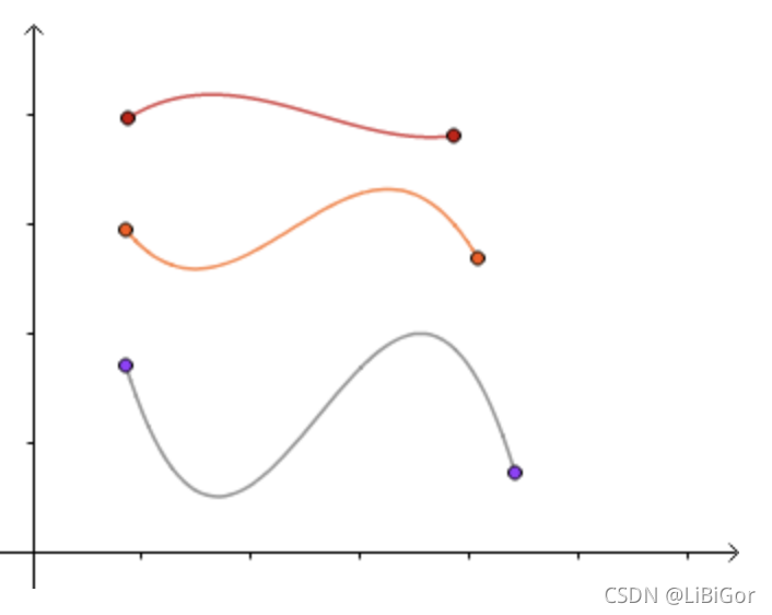 怎么来表示某一条曲线的弯曲程度呢?
我们知道三点确定一个圆:
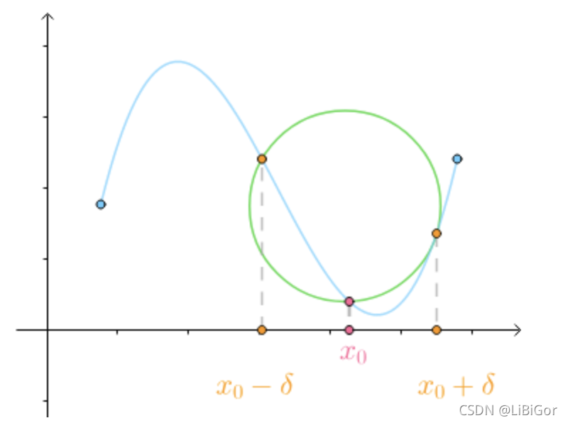
当δ 趋近于0时,我们可以的到曲线在x_0x0处的密切圆,也就是曲线在该点的圆近似:
另,在曲线比较平坦的位置,密切圆较大,在曲线比较弯曲的地方,密切圆较小,
因此,我们通过密切圆的曲率来定义曲线的曲率,定义如下:
二、实现
1.计算曲率半径的方法,代码实现如下:
代码如下(示例):
def cal_radius(img, left_fit, right_fit):
# 图像中像素个数与实际中距离的比率
# 沿车行进的方向长度大概覆盖了30米,按照美国高速公路的标准,宽度为3.7米(经验值)
ym_per_pix = 30 / 720
# y方向像素个数与距离的比例
xm_per_pix = 3.7 / 700
# x方向像素个数与距离的比例
# 计算得到曲线上的每个点
left_y_axis = np.linspace(0, img.shape[0], img.shape[0] - 1)
left_x_axis = left_fit[0] * left_y_axis ** 2 + left_fit[1] * left_y_axis + left_fit[2]
right_y_axis = np.linspace(0, img.shape[0], img.shape[0] - 1)
right_x_axis = right_fit[0] * right_y_axis ** 2 + right_fit[1] * right_y_axis + right_fit[2]
# 获取真实环境中的曲线
left_fit_cr = np.polyfit(left_y_axis * ym_per_pix, left_x_axis * xm_per_pix, 2)
right_fit_cr = np.polyfit(right_y_axis * ym_per_pix, right_x_axis * xm_per_pix, 2)
# 获得真实环境中的曲线曲率
left_curverad = ((1 + (2 * left_fit_cr[0] * left_y_axis * ym_per_pix + left_fit_cr[1]) ** 2) ** 1.5) / np.absolute(
2 * left_fit_cr[0])
right_curverad = ((1 + (
2 * right_fit_cr[0] * right_y_axis * ym_per_pix + right_fit_cr[1]) ** 2) ** 1.5) / np.absolute(
2 * right_fit_cr[0])
# 在图像上显示曲率
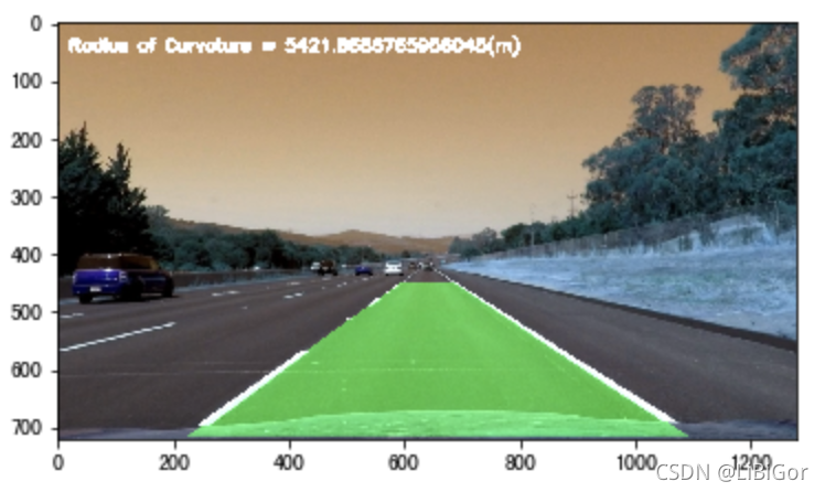
cv2.putText(img, 'Radius of Curvature = {}(m)'.format(np.mean(left_curverad)), (20, 50), cv2.FONT_ITALIC, 1,
(255, 255, 255), 5)
return img
曲率半径显示效果:
 计算偏离中心的距离:
# 1. 定义函数计算图像的中心点位置
def cal_line__center(img):
undistort_img = img_undistort(img, mtx, dist)
rigin_pipline_img = pipeline(undistort_img)
transform_img = img_perspect_transform(rigin_pipline_img, M)
left_fit, right_fit = cal_line_param(transform_img)
y_max = img.shape[0]
left_x = left_fit[0] * y_max ** 2 + left_fit[1] * y_max + left_fit[2]
right_x = right_fit[0] * y_max ** 2 + right_fit[1] * y_max + right_fit[2]
return (left_x + right_x) / 2
# 2. 假设straight_lines2_line.jpg,这张图片是位于车道的中央,实际情况可以根据测量验证.
img =cv2.imread("./test/straight_lines2_line.jpg")
lane_center = cal_line__center(img)
print("车道的中心点为:{}".format(lane_center))
# 3. 计算偏离中心的距离
def cal_center_departure(img, left_fit, right_fit):
# 计算中心点
y_max = img.shape[0]
left_x = left_fit[0] * y_max ** 2 + left_fit[1] * y_max + left_fit[2]
right_x = right_fit[0] * y_max ** 2 + right_fit[1] * y_max + right_fit[2]
xm_per_pix = 3.7 / 700
center_depart = ((left_x + right_x) / 2 - lane_center) * xm_per_pix
# 在图像上显示偏移
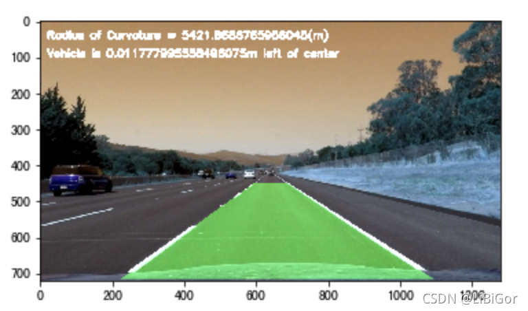
if center_depart > 0:
cv2.putText(img, 'Vehicle is {}m right of center'.format(center_depart), (20, 100), cv2.FONT_ITALIC, 1,
(255, 255, 255), 5)
elif center_depart < 0:
cv2.putText(img, 'Vehicle is {}m left of center'.format(-center_depart), (20, 100), cv2.FONT_ITALIC, 1,
(255, 255, 255), 5)
else:
cv2.putText(img, 'Vehicle is in the center', (20, 100), cv2.FONT_ITALIC, 1, (255, 255, 255), 5)
return img
计算偏离中心显示效果如下:
总结
曲率是表示曲线的弯曲程度,在这里是计算车道的弯曲程度
偏离中心的距离:利用已知的在中心的图像计算其他图像的偏离距离
# encoding:utf-8
from matplotlib import font_manager
my_font = font_manager.FontProperties(fname="/System/Library/Fonts/PingFang.ttc")
import cv2
import numpy as np
import matplotlib.pyplot as plt
#遍历文件夹
import glob
from moviepy.editor import VideoFileClip
import sys
reload(sys)
sys.setdefaultencoding('utf-8')
"""参数设置"""
nx = 9
ny = 6
#获取棋盘格数据
file_paths = glob.glob("./camera_cal/calibration*.jpg")
# # 绘制对比图
# def plot_contrast_image(origin_img, converted_img, origin_img_title="origin_img", converted_img_title="converted_img",
#
converted_img_gray=False):
#
fig, (ax1, ax2) = plt.subplots(1, 2, figsize=(15, 20))
#
ax1.set_title = origin_img_title
#
ax1.imshow(origin_img)
#
ax2.set_title = converted_img_title
#
if converted_img_gray == True:
#
ax2.imshow(converted_img, cmap="gray")
#
else:
#
ax2.imshow(converted_img)
#
plt.show()
#相机矫正使用opencv封装好的api
#目的:得到内参、外参、畸变系数
def cal_calibrate_params(file_paths):
#存储角点数据的坐标
object_points = [] #角点在真实三维空间的位置
image_points = [] #角点在图像空间中的位置
#生成角点在真实世界中的位置
objp = np.zeros((nx*ny,3),np.float32)
#以棋盘格作为坐标,每相邻的黑白棋的相差1
objp[:,:2] = np.mgrid[0:nx,0:ny].T.reshape(-1,2)
#角点检测
for file_path in file_paths:
img = cv2.imread(file_path)
#将图像灰度化
gray = cv2.cvtColor(img,cv2.COLOR_BGR2GRAY)
#角点检测
rect,coners = cv2.findChessboardCorners(gray,(nx,ny),None)
#若检测到角点,则进行保存 即得到了真实坐标和图像坐标
if rect == True :
object_points.append(objp)
image_points.append(coners)
# 相机较真
ret, mtx, dist, rvecs, tvecs = cv2.calibrateCamera(object_points, image_points, gray.shape[::-1], None, None)
return ret, mtx, dist, rvecs, tvecs
# 图像去畸变:利用相机校正的内参,畸变系数
def img_undistort(img, mtx, dist):
dis = cv2.undistort(img, mtx, dist, None, mtx)
return dis
#车道线提取
#颜色空间转换--》边缘检测--》颜色阈值--》并且使用L通道进行白色的区域进行抑制
def pipeline(img,s_thresh = (170,255),sx_thresh=(40,200)):
# 复制原图像
img = np.copy(img)
# 颜色空间转换
hls = cv2.cvtColor(img,cv2.COLOR_RGB2HLS).astype(np.float)
l_chanel = hls[:,:,1]
s_chanel = hls[:,:,2]
#sobel边缘检测
sobelx = cv2.Sobel(l_chanel,cv2.CV_64F,1,0)
#求绝对值
abs_sobelx = np.absolute(sobelx)
#将其转换为8bit的整数
scaled_sobel = np.uint8(255 * abs_sobelx / np.max(abs_sobelx))
#对边缘提取的结果进行二值化
sxbinary = np.zeros_like(scaled_sobel)
#边缘位置赋值为1,非边缘位置赋值为0
sxbinary[(scaled_sobel >= sx_thresh[0]) & (scaled_sobel <= sx_thresh[1])] = 1
#对S通道进行阈值处理
s_binary = np.zeros_like(s_chanel)
s_binary[(s_chanel >= s_thresh[0]) & (s_chanel <= s_thresh[1])] = 1
# 结合边缘提取结果和颜色通道的结果,
color_binary = np.zeros_like(sxbinary)
color_binary[((sxbinary == 1) | (s_binary == 1)) & (l_chanel > 100)] = 1
return color_binary
#透视变换-->将检测结果转换为俯视图。
#获取透视变换的参数矩阵【二值图的四个点】
def cal_perspective_params(img,points):
# x与y方向上的偏移
offset_x = 330
offset_y = 0
#转换之后img的大小
img_size = (img.shape[1],img.shape[0])
src = np.float32(points)
#设置俯视图中的对应的四个点 左上角 右上角 左下角 右下角
dst = np.float32([[offset_x, offset_y], [img_size[0] - offset_x, offset_y],
[offset_x, img_size[1] - offset_y], [img_size[0] - offset_x, img_size[1] - offset_y]])
## 原图像转换到俯视图
M = cv2.getPerspectiveTransform(src, dst)
# 俯视图到原图像
M_inverse = cv2.getPerspectiveTransform(dst, src)
return M, M_inverse
#根据透视变化矩阵完成透视变换
def img_perspect_transform(img,M):
#获取图像大小
img_size = (img.shape[1],img.shape[0])
#完成图像的透视变化
return cv2.warpPerspective(img,M,img_size)
# 精确定位车道线
#传入已经经过边缘检测的图像阈值结果的二值图,再进行透明变换
def cal_line_param(binary_warped):
#定位车道线的大致位置==计算直方图
histogram = np.sum(binary_warped[:,:],axis=0) #计算y轴
# 将直方图一分为二,分别进行左右车道线的定位
midpoint = np.int(histogram.shape[0]/2)
#分别统计左右车道的最大值
midpoint = np.int(histogram.shape[0] / 2)
leftx_base = np.argmax(histogram[:midpoint]) #左车道
rightx_base = np.argmax(histogram[midpoint:]) + midpoint #右车道
#设置滑动窗口
#对每一个车道线来说 滑动窗口的个数
nwindows = 9
#设置滑动窗口的高
window_height = np.int(binary_warped.shape[0]/nwindows)
#设置滑动窗口的宽度==x的检测范围,即滑动窗口的一半
margin = 100
#统计图像中非0点的个数
nonzero = binary_warped.nonzero()
nonzeroy = np.array(nonzero[0])#非0点的位置-x坐标序列
nonzerox = np.array(nonzero[1])#非0点的位置-y坐标序列
#车道检测位置
leftx_current = leftx_base
rightx_current = rightx_base
#设置阈值:表示当前滑动窗口中的非0点的个数
minpix = 50
#记录窗口中,非0点的索引
left_lane_inds = []
right_lane_inds = []
#遍历滑动窗口
for window in range(nwindows):
# 设置窗口的y的检测范围,因为图像是(行列),shape[0]表示y方向的结果,上面是0
win_y_low = binary_warped.shape[0] - (window + 1) * window_height #y的最低点
win_y_high = binary_warped.shape[0] - window * window_height #y的最高点
# 左车道x的范围
win_xleft_low = leftx_current - margin
win_xleft_high = leftx_current + margin
# 右车道x的范围
win_xright_low = rightx_current - margin
win_xright_high = rightx_current + margin
# 确定非零点的位置x,y是否在搜索窗口中,将在搜索窗口内的x,y的索引存入left_lane_inds和right_lane_inds中
good_left_inds = ((nonzeroy >= win_y_low) & (nonzeroy < win_y_high) &
(nonzerox >= win_xleft_low) & (nonzerox < win_xleft_high)).nonzero()[0]
good_right_inds = ((nonzeroy >= win_y_low) & (nonzeroy < win_y_high) &
(nonzerox >= win_xright_low) & (nonzerox < win_xright_high)).nonzero()[0]
left_lane_inds.append(good_left_inds)
right_lane_inds.append(good_right_inds)
# 如果获取的点的个数大于最小个数,则利用其更新滑动窗口在x轴的位置=修正车道线的位置
if len(good_left_inds) > minpix:
leftx_current = np.int(np.mean(nonzerox[good_left_inds]))
if len(good_right_inds) > minpix:
rightx_current = np.int(np.mean(nonzerox[good_right_inds]))
# 将检测出的左右车道点转换为array
left_lane_inds = np.concatenate(left_lane_inds)
right_lane_inds = np.concatenate(right_lane_inds)
# 获取检测出的左右车道x与y点在图像中的位置
leftx = nonzerox[left_lane_inds]
lefty = nonzeroy[left_lane_inds]
rightx = nonzerox[right_lane_inds]
righty = nonzeroy[right_lane_inds]
# 3.用曲线拟合检测出的点,二次多项式拟合,返回的结果是系数
left_fit = np.polyfit(lefty, leftx, 2)
right_fit = np.polyfit(righty, rightx, 2)
return left_fit, right_fit
#填充车道线之间的多边形
def fill_lane_poly(img,left_fit,right_fit):
#行数
y_max = img.shape[0]
#设置填充之后的图像的大小 取到0-255之间
out_img = np.dstack((img,img,img))*255
#根据拟合结果,获取拟合曲线的车道线像素位置
left_points = [[left_fit[0] * y ** 2 + left_fit[1] * y + left_fit[2], y] for y in range(y_max)]
right_points = [[right_fit[0] * y ** 2 + right_fit[1] * y + right_fit[2], y] for y in range(y_max - 1, -1, -1)]
# 将左右车道的像素点进行合并
line_points = np.vstack((left_points, right_points))
# 根据左右车道线的像素位置绘制多边形
cv2.fillPoly(out_img, np.int_([line_points]), (0, 255, 0))
return out_img
#计算车道线曲率的方法
def cal_readius(img,left_fit,right_fit):
# 比例
ym_per_pix = 30/720
xm_per_pix = 3.7/700
# 得到车道线上的每个点
left_y_axis = np.linspace(0,img.shape[0],img.shape[0]-1) #个数img.shape[0]-1
left_x_axis = left_fit[0]*left_y_axis**2+left_fit[1]*left_y_axis+left_fit[0]
right_y_axis = np.linspace(0,img.shape[0],img.shape[0]-1)
right_x_axis = right_fit[0]*right_y_axis**2+right_fit[1]*right_y_axis+right_fit[2]
# 把曲线中的点映射真实世界,再计算曲率
left_fit_cr = np.polyfit(left_y_axis*ym_per_pix,left_x_axis*xm_per_pix,2)
right_fit_cr = np.polyfit(right_y_axis*ym_per_pix,right_x_axis*xm_per_pix,2)
# 计算曲率
left_curverad = ((1+(2*left_fit_cr[0]*left_y_axis*ym_per_pix+left_fit_cr[1])**2)**1.5)/np.absolute(2*left_fit_cr[0])
right_curverad = ((1+(2*right_fit_cr[0]*right_y_axis*ym_per_pix *right_fit_cr[1])**2)**1.5)/np.absolute((2*right_fit_cr[0]))
# 将曲率半径渲染在图像上 写什么
cv2.putText(img,'Radius of Curvature = {}(m)'.format(np.mean(left_curverad)),(20,50),cv2.FONT_ITALIC,1,(255,255,255),5)
return img
# 计算车道线中心的位置
def cal_line_center(img):
#去畸变
undistort_img = img_undistort(img,mtx,dist)
#提取车道线
rigin_pipeline_img = pipeline(undistort_img)
#透视变换
trasform_img = img_perspect_transform(rigin_pipeline_img,M)
#精确定位
left_fit,right_fit = cal_line_param(trasform_img)
#当前图像的shape[0]
y_max = img.shape[0]
#左车道线
left_x = left_fit[0]*y_max**2+left_fit[1]*y_max+left_fit[2]
#右车道线
right_x = right_fit[0]*y_max**2+right_fit[1]*y_max+right_fit[2]
#返回车道中心点
return (left_x+right_x)/2
def cal_center_departure(img,left_fit,right_fit):
# 计算中心点
y_max = img.shape[0]
left_x = left_fit[0]*y_max**2 + left_fit[1]*y_max +left_fit[2]
right_x = right_fit[0]*y_max**2 +right_fit[1]*y_max +right_fit[2]
xm_per_pix = 3.7/700
center_depart = ((left_x+right_x)/2-lane_center)*xm_per_pix
# 渲染
if center_depart>0:
cv2.putText(img,'Vehicle is {}m right of center'.format(center_depart), (20, 100), cv2.FONT_ITALIC, 1,
(255, 255, 255), 5)
elif center_depart<0:
cv2.putText(img, 'Vehicle is {}m left of center'.format(-center_depart), (20, 100), cv2.FONT_ITALIC, 1,
(255, 255, 255), 5)
else:
cv2.putText(img, 'Vehicle is in the center', (20, 100), cv2.FONT_ITALIC, 1, (255, 255, 255), 5)
return img
#计算车辆偏离中心点的距离
def cal_center_departure(img,left_fit,right_fit):
# 计算中心点
y_max = img.shape[0]
#左车道线
left_x = left_fit[0]*y_max**2 + left_fit[1]*y_max +left_fit[2]
#右车道线
right_x = right_fit[0]*y_max**2 +right_fit[1]*y_max +right_fit[2]
#x方向上每个像素点代表的距离大小
xm_per_pix = 3.7/700
#计算偏移距离 像素距离 × xm_per_pix = 实际距离
center_depart = ((left_x+right_x)/2-lane_center)*xm_per_pix
# 渲染
if center_depart>0:
cv2.putText(img,'Vehicle is {}m right of center'.format(center_depart), (20, 100), cv2.FONT_ITALIC, 1,
(255, 255, 255), 5)
elif center_depart<0:
cv2.putText(img, 'Vehicle is {}m left of center'.format(-center_depart), (20, 100), cv2.FONT_ITALIC, 1,
(255, 255, 255), 5)
else:
cv2.putText(img, 'Vehicle is in the center', (20, 100), cv2.FONT_ITALIC, 1, (255, 255, 255), 5)
return img
if __name__ == "__main__":
ret, mtx, dist, rvecs, tvecs = cal_calibrate_params(file_paths)
#透视变换
#获取原图的四个点
img = cv2.imread('./test/straight_lines2.jpg')
points = [[601, 448], [683, 448], [230, 717], [1097, 717]]
#将四个点绘制到图像上 (文件,坐标起点,坐标终点,颜色,连接起来)
img = cv2.line(img, (601, 448), (683, 448), (0, 0, 255), 3)
img = cv2.line(img, (683, 448), (1097, 717), (0, 0, 255), 3)
img = cv2.line(img, (1097, 717), (230, 717), (0, 0, 255), 3)
img = cv2.line(img, (230, 717), (601, 448), (0, 0, 255), 3)
#透视变换的矩阵
M,M_inverse = cal_perspective_params(img,points)
#计算车道线的中心距离
lane_center = cal_line_center(img)
最后
以上就是复杂电话最近收集整理的关于自动驾驶道路曲率计算自动驾驶系列目标一、曲率的介绍二、实现的全部内容,更多相关自动驾驶道路曲率计算自动驾驶系列目标一、曲率内容请搜索靠谱客的其他文章。
本图文内容来源于网友提供,作为学习参考使用,或来自网络收集整理,版权属于原作者所有。


发表评论 取消回复