An Introduction to Gradient Descent and Linear Regression
Gradient descent is one of those “greatest hits” algorithms that can offer a new perspective for solving problems. Unfortunately, it’s rarely taught in undergraduate computer science programs. In this post I’ll give an introduction to the gradient descent algorithm, and walk through an example that demonstrates how gradient descent can be used to solve machine learning problems such as linear regression.
At a theoretical level, gradient descent is an algorithm that minimizes functions. Given a function defined by a set of parameters, gradient descent starts with an initial set of parameter values and iteratively moves toward a set of parameter values that minimize the function. This iterative minimization is achieved using calculus, taking steps in the negative direction of the function gradient.
It’s sometimes difficult to see how this mathematical explanation translates into a practical setting, so it’s helpful to look at an example. The canonical example when explaining gradient descent is linear regression.
Code for this example can be found here
Linear Regression Example
Simply stated, the goal of linear regression is to fit a line to a set of points. Consider the following data.
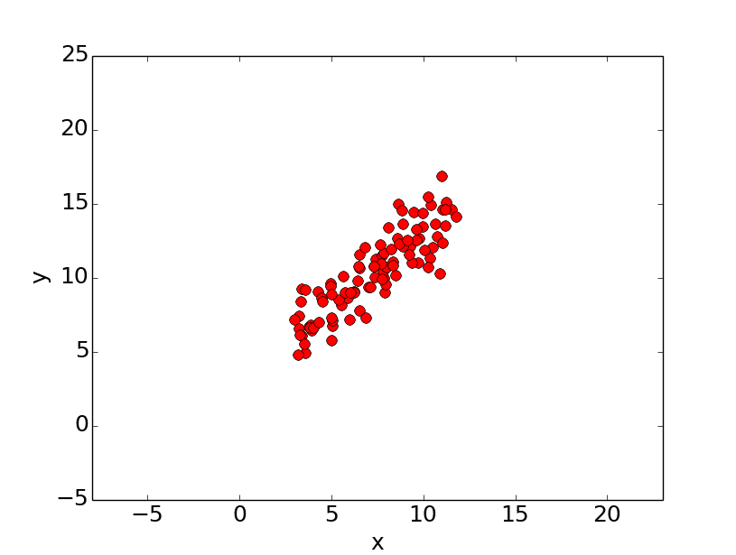
Let’s suppose we want to model the above set of points with a line. To do this we’ll use the standard y = mx + b line equation where m is the line’s slope and b is the line’s y-intercept. To find the best line for our data, we need to find the best set of slope m and y-intercept b values.
A standard approach to solving this type of problem is to define an error function (also called a cost function) that measures how “good” a given line is. This function will take in a (m,b) pair and return an error value based on how well the line fits our data. To compute this error for a given line, we’ll iterate through each (x,y) point in our data set and sum the square distances between each point’s y value and the candidate line’s y value (computed at mx + b). It’s conventional to square this distance to ensure that it is positive and to make our error function differentiable. In python, computing the error for a given line will look like:
# y = mx + b
# m is slope, b is y-intercept
def computeErrorForLineGivenPoints(b, m, points):
    totalError = 0
    for i in range(0, len(points)):
        totalError += (points[i].y - (m * points[i].x + b)) ** 2
    return totalError / float(len(points))
Formally, this error function looks like:
Lines that fit our data better (where better is defined by our error function) will result in lower error values. If we minimize this function, we will get the best line for our data. Since our error function consists of two parameters (m and b) we can visualize it as a two-dimensional surface. This is what it looks like for our data set:
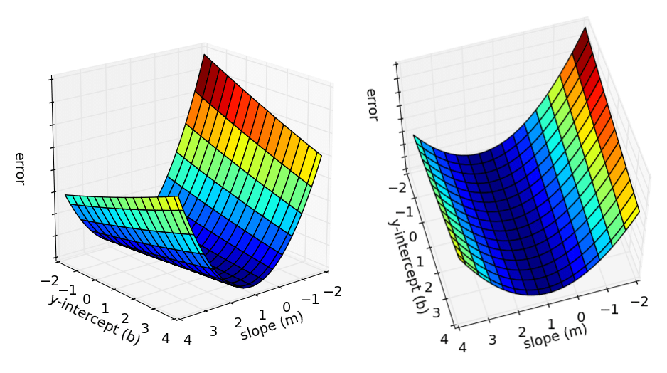
Each point in this two-dimensional space represents a line. The height of the function at each point is the error value for that line. You can see that some lines yield smaller error values than others (i.e., fit our data better). When we run gradient descent search, we will start from some location on this surface and move downhill to find the line with the lowest error.
To run gradient descent on this error function, we first need to compute its gradient. The gradient will act like a compass and always point us downhill. To compute it, we will need to differentiate our error function. Since our function is defined by two parameters (m and b), we will need to compute a partial derivative for each. These derivatives work out to be:
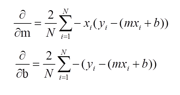
We now have all the tools needed to run gradient descent. We can initialize our search to start at any pair of m and b values (i.e., any line) and let the gradient descent algorithm march downhill on our error function towards the best line. Each iteration will update m and b to a line that yields slightly lower error than the previous iteration. The direction to move in for each iteration is calculated using the two partial derivatives from above and looks like this:
def stepGradient(b_current, m_current, points, learningRate):
    b_gradient = 0
    m_gradient = 0
    N = float(len(points))
    for i in range(0, len(points)):
        b_gradient += -(2/N) * (points[i].y - ((m_current*points[i].x) + b_current))
        m_gradient += -(2/N) * points[i].x * (points[i].y - ((m_current * points[i].x) + b_current))
    new_b = b_current - (learningRate * b_gradient)
    new_m = m_current - (learningRate * m_gradient)
    return [new_b, new_m]
The learningRate variable controls how large of a step we take downhill during each iteration. If we take too large of a step, we may step over the minimum. However, if we take small steps, it will require many iterations to arrive at the minimum.
Below are some snapshots of gradient descent running for 2000 iterations for our example problem. We start out at point m = -1 b = 0. Each iteration m and b are updated to values that yield slightly lower error than the previous iteration. The left plot displays the current location of the gradient descent search (blue dot) and the path taken to get there (black line). The right plot displays the corresponding line for the current search location. Eventually we ended up with a pretty accurate fit.

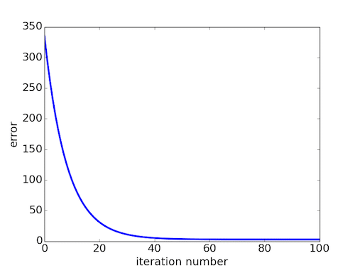
We can also observe how the error changes as we move toward the minimum. A good way to ensure that gradient descent is working correctly is to make sure that the error decreases for each iteration. Below is a plot of error values for the first 100 iterations of the above gradient search.
We’ve now seen how gradient descent can be applied to solve a linear regression problem. While the model in our example was a line, the concept of minimizing a cost function to tune parameters also applies to regression problems that use higher order polynomials and other problems found around the machine learning world.
While we were able to scratch the surface for learning gradient descent, there are several additional concepts that are good to be aware of that we weren’t able to discuss. A few of these include:
- Convexity – In our linear regression problem, there was only one minimum. Our error surface was convex. Regardless of where we started, we would eventually arrive at the absolute minimum. In general, this need not be the case. It’s possible to have a problem with local minima that a gradient search can get stuck in. There are several approaches to mitigate this (e.g., stochastic gradient search).
- Performance – We used vanilla gradient descent with a learning rate of 0.0005 in the above example, and ran it for 2000 iterations. There are approaches such a line search, that can reduce the number of iterations required. For the above example, line search reduces the number of iterations to arrive at a reasonable solution from several thousand to around 50.
- Convergence – We didn’t talk about how to determine when the search finds a solution. This is typically done by looking for small changes in error iteration-to-iteration (e.g., where the gradient is near zero).
For more information about gradient descent, linear regression, and other machine learning topics, I would strongly recommend Andrew Ng’s machine learning course on Coursera.
Example Code
Example code for the problem described above can be found here
Edit: I chose to use linear regression example above for simplicity. We used gradient descent to iteratively estimate m and b, however we could have also solved for them directly. My intention was to illustrate how gradient descent can be used to iteratively estimate/tune parameters, as this is required for many different problems in machine learning.
代码实现:
from numpy import *

# y = mx + b
# m is slope, b is y-intercept
def compute_error_for_line_given_points(b, m, points):
    totalError = 0
    for i in range(0, len(points)):
        x = points[i, 0]
        y = points[i, 1]
        totalError += (y - (m * x + b)) ** 2
    return totalError / float(len(points))

def step_gradient(b_current, m_current, points, learningRate):
    b_gradient = 0
    m_gradient = 0
    N = float(len(points))
    for i in range(0, len(points)):
        x = points[i, 0]
        y = points[i, 1]
        b_gradient += -(2/N) * (y - ((m_current * x) + b_current))
        m_gradient += -(2/N) * x * (y - ((m_current * x) + b_current))
    new_b = b_current - (learningRate * b_gradient)
    new_m = m_current - (learningRate * m_gradient)
    return [new_b, new_m]

def gradient_descent_runner(points, starting_b, starting_m, learning_rate, num_iterations):
    b = starting_b
    m = starting_m
    for i in range(num_iterations):
        b, m = step_gradient(b, m, array(points), learning_rate)
    return [b, m]

def run():
    points = genfromtxt("data.csv", delimiter=",")
    learning_rate = 0.0001
    initial_b = 0 # initial y-intercept guess
    initial_m = 0 # initial slope guess
    num_iterations = 1000
    print("Starting gradient descent at b = {0}, m = {1}, error = {2}".format(initial_b, initial_m, compute_error_for_line_given_points(initial_b, initial_m, points)))
    print("Running...")
    [b, m] = gradient_descent_runner(points, initial_b, initial_m, learning_rate, num_iterations)
    print("After {0} iterations b = {1}, m = {2}, error = {3}".format(num_iterations, b, m, compute_error_for_line_given_points(b, m, points)))

if __name__ == '__main__':
    run()
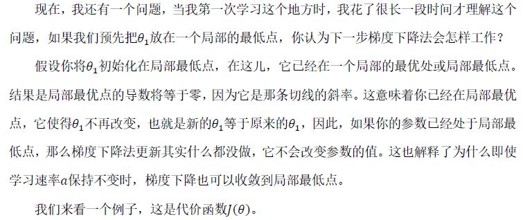
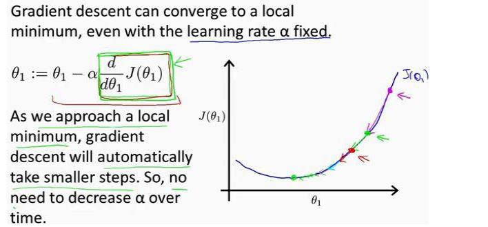
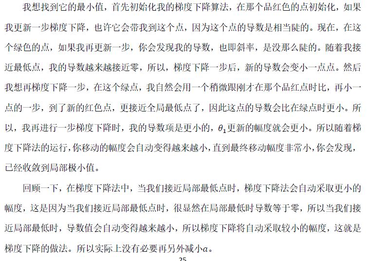
刚学习的梯度下降法的时候,看到前面的代码,一直纳闷难道不需要一个收敛判断条件判断获取的误差是否达到最小值?查看《机器学习个人笔记完整版》才知道梯度下降的时候,它会根据梯度大小自动收敛于一个局部最小值,并不需要额外的进行判断是否收敛到了局部最小值。由于局部最小值可能并不是全局最小值,那么为了找到全局最小值,我们可以多个初始值开始进行梯度收敛,从多个初始值收敛寻找几个局部最小值的最小值即为全局最小值。
文章出处:An Introduction to Gradient Descent and Linear Regression
参考资料:机器学习个人笔记完整版
最后
以上就是激昂柠檬最近收集整理的关于An Introduction to Gradient Descent and Linear Regression--梯度下降法和线性回归介绍An Introduction to Gradient Descent and Linear Regression 的全部内容,更多相关An内容请搜索靠谱客的其他文章。


发表评论 取消回复