Cat vs. Dog Image Classification

练习1：从头构建一个卷积网络

• ** 预计完成时间：20分钟 **

在本练习中，我们将从头开始构建一个能够区分狗和猫的分类器模型。 我们将遵循以下步骤：

1.探索示例数据
2.从头开始构建一个小小的网站来解决我们的分类问题
3.评估培训和验证准确性

Let’s go!

探索示例数据

让我们首先下载我们的示例数据，一个包含2000张JPG猫狗照片的.zip，并在/ tmp中本地提取它。
**注意：**本练习中使用的2,000张图片摘自Kaggle提供的[“Dogs vs. Cats”数据集]（https://www.kaggle.com/c/dogs-vs-cats/data） ，其中包含25,000张图片。 在这里，我们使用完整数据集的子集来减少用于教育目的的培训时间。

!wget --no-check-certificate 
    https://storage.googleapis.com/mledu-datasets/cats_and_dogs_filtered.zip 
    -O /tmp/cats_and_dogs_filtered.zip

import os
import zipfile

local_zip = '/tmp/cats_and_dogs_filtered.zip'
zip_ref = zipfile.ZipFile(local_zip, 'r')
zip_ref.extractall('/tmp')
zip_ref.close()

.zip的内容被提取到基本目录/ tmp / cats_and_dogs_filtered，其中包含train和validation
培训和验证数据集的子目录（参见[机器学习速成课程]（https://developers.google.com/machine-learning/crash-course/validation/check-your-intuition）进行培训复习，
验证和测试集），每个都包含cats和dogs子目录。 让我们定义每个目录：

base_dir = '/tmp/cats_and_dogs_filtered'
train_dir = os.path.join(base_dir, 'train')
validation_dir = os.path.join(base_dir, 'validation')

# Directory with our training cat pictures
train_cats_dir = os.path.join(train_dir, 'cats')

# Directory with our training dog pictures
train_dogs_dir = os.path.join(train_dir, 'dogs')

# Directory with our validation cat pictures
validation_cats_dir = os.path.join(validation_dir, 'cats')

# Directory with our validation dog pictures
validation_dogs_dir = os.path.join(validation_dir, 'dogs')

现在，让我们看看cats和dogs``train目录中的文件名是什么样的（文件命名约定在validation目录中是相同的）：

train_cat_fnames = os.listdir(train_cats_dir)
print train_cat_fnames[:10]

train_dog_fnames = os.listdir(train_dogs_dir)
train_dog_fnames.sort()
print train_dog_fnames[:10]

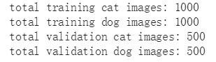
让我们找出train和validation目录中cat和dog图像的总数：

print 'total training cat images:', len(os.listdir(train_cats_dir))
print 'total training dog images:', len(os.listdir(train_dogs_dir))
print 'total validation cat images:', len(os.listdir(validation_cats_dir))
print 'total validation dog images:', len(os.listdir(validation_dogs_dir))

对于猫和狗，我们有1,000个训练图像和500个测试图像。

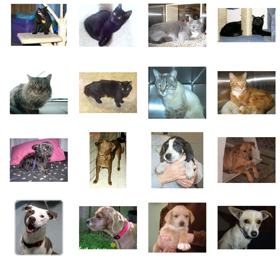
现在让我们看看几张图片，以便更好地了解猫狗数据集的外观。 首先，配置matplot参数：

%matplotlib inline

import matplotlib.pyplot as plt
import matplotlib.image as mpimg

# Parameters for our graph; we'll output images in a 4x4 configuration
nrows = 4
ncols = 4

# Index for iterating over images
pic_index = 0

现在，显示一批8只猫和8只狗图片。 您可以重新运行单元格以查看每次新批次：

# Set up matplotlib fig, and size it to fit 4x4 pics
fig = plt.gcf()
fig.set_size_inches(ncols * 4, nrows * 4)

pic_index += 8
next_cat_pix = [os.path.join(train_cats_dir, fname) 
                for fname in train_cat_fnames[pic_index-8:pic_index]]
next_dog_pix = [os.path.join(train_dogs_dir, fname) 
                for fname in train_dog_fnames[pic_index-8:pic_index]]

for i, img_path in enumerate(next_cat_pix+next_dog_pix):
  # Set up subplot; subplot indices start at 1
  sp = plt.subplot(nrows, ncols, i + 1)
  sp.axis('Off') # Don't show axes (or gridlines)

  img = mpimg.imread(img_path)
  plt.imshow(img)

plt.show()

从头开始构建小型Convnet以达到72％的准确率

将进入我们的网站的图像是150x150彩色图像（在下一节数据预处理中，我们将添加处理以将所有图像调整为150x150，然后将它们输入神经网络）。

让我们编写架构代码。 我们将堆叠3个{convolution + relu + maxpooling}模块。 我们的卷积在3x3窗口上运行，我们的maxpooling层在2x2窗口上运行。 我们的第一个卷积提取16个滤波器，下面一个提取32个滤波器，最后一个提取64个滤波器。

注意：这是一种广泛使用的配置，并且已知可以很好地用于图像分类。 此外，由于我们只有相对较少的训练样例（1,000），仅使用三个卷积模块可以保持模型小，从而降低过度拟合的风险（我们将在练习2中更深入地探讨）。

from tensorflow.keras import layers
from tensorflow.keras import Model

# Our input feature map is 150x150x3: 150x150 for the image pixels, and 3 for
# the three color channels: R, G, and B
img_input = layers.Input(shape=(150, 150, 3))

# First convolution extracts 16 filters that are 3x3
# Convolution is followed by max-pooling layer with a 2x2 window
x = layers.Conv2D(16, 3, activation='relu')(img_input)
x = layers.MaxPooling2D(2)(x)

# Second convolution extracts 32 filters that are 3x3
# Convolution is followed by max-pooling layer with a 2x2 window
x = layers.Conv2D(32, 3, activation='relu')(x)
x = layers.MaxPooling2D(2)(x)

# Third convolution extracts 64 filters that are 3x3
# Convolution is followed by max-pooling layer with a 2x2 window
x = layers.Conv2D(64, 3, activation='relu')(x)
x = layers.MaxPooling2D(2)(x)

最重要的是，我们粘贴了两个完全连接的层。 因为我们正面临一个两类分类问题，即二元分类问题，我们将以[* sigmoid * activation]（https://wikipedia.org/wiki/Sigmoid_function）结束我们的网络，以便输出 我们的网络将是0和1之间的单个标量，编码当前图像为1级（而不是0级）的概率。

# Flatten feature map to a 1-dim tensor so we can add fully connected layers
x = layers.Flatten()(x)

# Create a fully connected layer with ReLU activation and 512 hidden units
x = layers.Dense(512, activation='relu')(x)

# Create output layer with a single node and sigmoid activation
output = layers.Dense(1, activation='sigmoid')(x)

# Create model:
# input = input feature map
# output = input feature map + stacked convolution/maxpooling layers + fully 
# connected layer + sigmoid output layer
model = Model(img_input, output)

下面总结一下模型结构：

model.summary()

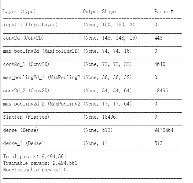
“输出形状”列显示特征贴图的大小如何在每个连续图层中演变。由于填充，卷积层将特征映射的大小减少一点，并且每个池化层将特征映射减半。
接下来，我们将配置模型培训的规范。我们将使用binary_crossentropy损失训练我们的模型，因为它是二进制分类问题，我们的最终激活是一个sigmoid。 （有关损失指标的更新，请参阅[机器学习速成课程]（https://developers.google.com/machine-learning/crash-course/descending-into-ml/video-lecture）。）我们将使用rmsprop优化器，学习率为0.001。在培训期间，我们希望监控分类准确性。

注意：在这种情况下，使用[RMSprop优化算法]（https://wikipedia.org/wiki/Stochastic_gradient_descent#RMSProp）优于[随机梯度下降]（https://developers.google.com / machine-learning / glossary /＃SGD）（SGD），因为RMSprop为我们自动化学习速率调整。 （其他优化器，如[Adam]（https://wikipedia.org/wiki/Stochastic_gradient_descent#Adam）和[Adagrad]（https://developers.google.com/machine-learning/glossary/#AdaGrad），在培训期间自动调整学习率，并在这里同样有效。）

from tensorflow.keras.optimizers import RMSprop

model.compile(loss='binary_crossentropy',
              optimizer=RMSprop(lr=0.001),
              metrics=['acc'])

数据预处理

让我们设置数据生成器，它将读取源文件夹中的图片，将它们转换为float32张量，并将它们（及其标签）提供给我们的网络。我们将有一个用于训练图像的生成器和一个用于验证图像的生成器。我们的发电机将生产20个尺寸为150x150的图像及其标签（二进制）。

您可能已经知道，进入神经网络的数据通常应该以某种方式进行标准化，以使其更适合网络处理。 （将原始像素输入到一个回旋网中是不常见的。）在我们的例子中，我们将通过将像素值归一化到“[0,1]”范围来预处理我们的图像（最初所有值都在[0， 255]范围）。

在Keras中，可以使用rescale参数通过keras.preprocessing.image.ImageDataGenerator类完成。这个ImageDataGenerator类允许你通过.flow（data，labels）或.flow_from_directory（directory）来实例化增强图像批次（及其标签）的生成器。然后，这些生成器可以与接受数据生成器作为输入的Keras模型方法一起使用：fit_generator，evaluate_generator和predict_generator。

from tensorflow.keras.preprocessing.image import ImageDataGenerator

# All images will be rescaled by 1./255
train_datagen = ImageDataGenerator(rescale=1./255)
test_datagen = ImageDataGenerator(rescale=1./255)

# Flow training images in batches of 20 using train_datagen generator
train_generator = train_datagen.flow_from_directory(
        train_dir,  # This is the source directory for training images
        target_size=(150, 150),  # All images will be resized to 150x150
        batch_size=20,
        # Since we use binary_crossentropy loss, we need binary labels
        class_mode='binary')

# Flow validation images in batches of 20 using test_datagen generator
validation_generator = test_datagen.flow_from_directory(
        validation_dir,
        target_size=(150, 150),
        batch_size=20,
        class_mode='binary')

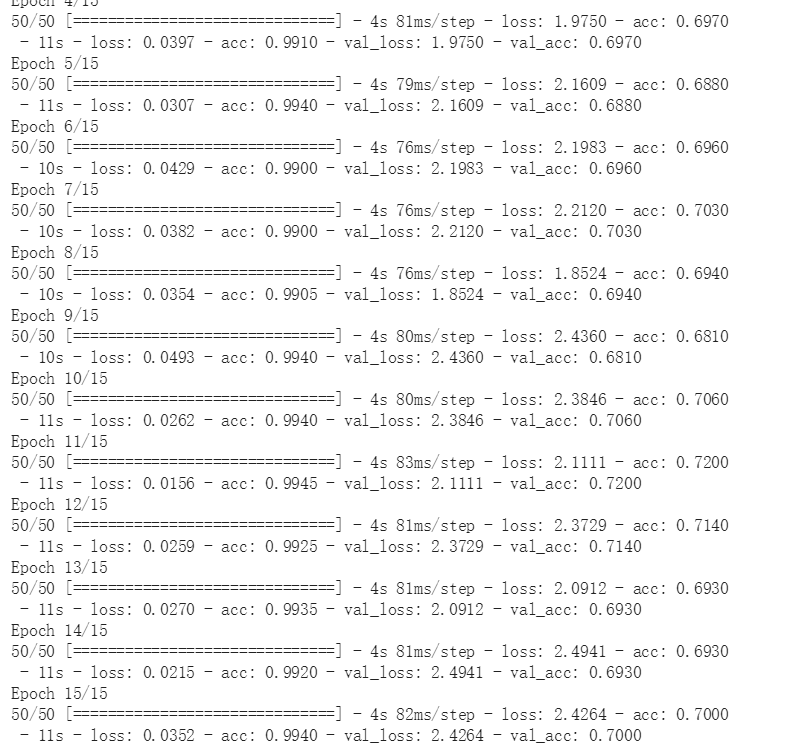
Training

让我们训练所有2000个可用的图像，共15个时期，并验证所有1,000个测试图像。 （这可能需要几分钟才能运行。）

history = model.fit_generator(
      train_generator,
      steps_per_epoch=100,  # 2000 images = batch_size * steps
      epochs=15,
      validation_data=validation_generator,
      validation_steps=50,  # 1000 images = batch_size * steps
      verbose=2)

可视化中间表示

为了了解我们的网站所学习的功能，一个有趣的事情是可视化输入在通过网络传输时如何变换。

让我们从训练集中选择一个随机的猫或狗图像，然后生成一个图形，其中每一行是图层的输出，并且该行中的每个图像都是该输出特征图中的特定滤镜。 重新运行此单元格以生成各种训练图像的中间表示。

import numpy as np
import random
from tensorflow.keras.preprocessing.image import img_to_array, load_img

# Let's define a new Model that will take an image as input, and will output
# intermediate representations for all layers in the previous model after
# the first.
successive_outputs = [layer.output for layer in model.layers[1:]]
visualization_model = Model(img_input, successive_outputs)

# Let's prepare a random input image of a cat or dog from the training set.
cat_img_files = [os.path.join(train_cats_dir, f) for f in train_cat_fnames]
dog_img_files = [os.path.join(train_dogs_dir, f) for f in train_dog_fnames]
img_path = random.choice(cat_img_files + dog_img_files)

img = load_img(img_path, target_size=(150, 150))  # this is a PIL image
x = img_to_array(img)  # Numpy array with shape (150, 150, 3)
x = x.reshape((1,) + x.shape)  # Numpy array with shape (1, 150, 150, 3)

# Rescale by 1/255
x /= 255

# Let's run our image through our network, thus obtaining all
# intermediate representations for this image.
successive_feature_maps = visualization_model.predict(x)

# These are the names of the layers, so can have them as part of our plot
layer_names = [layer.name for layer in model.layers]

# Now let's display our representations
for layer_name, feature_map in zip(layer_names, successive_feature_maps):
  if len(feature_map.shape) == 4:
    # Just do this for the conv / maxpool layers, not the fully-connected layers
    n_features = feature_map.shape[-1]  # number of features in feature map
    # The feature map has shape (1, size, size, n_features)
    size = feature_map.shape[1]
    # We will tile our images in this matrix
    display_grid = np.zeros((size, size * n_features))
    for i in range(n_features):
      # Postprocess the feature to make it visually palatable
      x = feature_map[0, :, :, i]
      x -= x.mean()
      x /= x.std()
      x *= 64
      x += 128
      x = np.clip(x, 0, 255).astype('uint8')
      # We'll tile each filter into this big horizontal grid
      display_grid[:, i * size : (i + 1) * size] = x
    # Display the grid
    scale = 20. / n_features
    plt.figure(figsize=(scale * n_features, scale))
    plt.title(layer_name)
    plt.grid(False)
    plt.imshow(display_grid, aspect='auto', cmap='viridis')

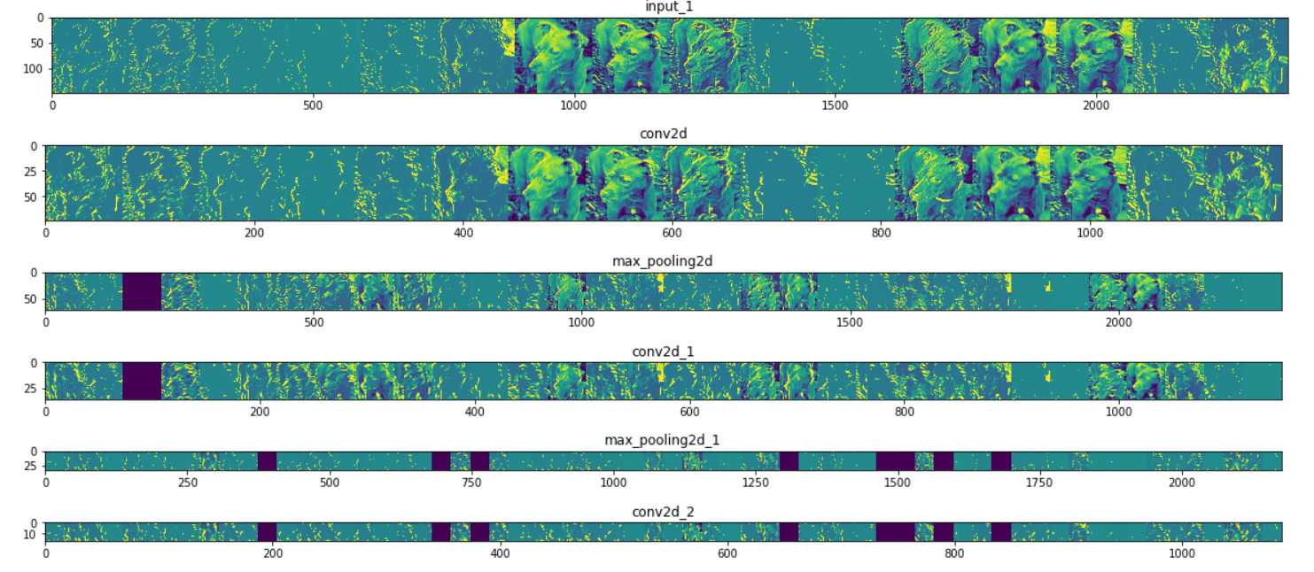
正如您所看到的，我们从图像的原始像素变为越来越抽象和紧凑的表示。 下游的表示开始突出显示网络关注的内容，并且它们显示越来越少的功能被“激活”; 大多数都设置为零。 这被称为“稀疏性”。 表示稀疏性是深度学习的关键特征。

这些表示关于图像的原始像素的信息越来越少，但是关于图像类别的信息越来越精细。 您可以将convnet（或一般的深层网络）视为信息蒸馏管道。

Evaluating Accuracy and Loss for the Model

Let’s plot the training/validation accuracy and loss as collected during training:

# Retrieve a list of accuracy results on training and test data
# sets for each training epoch
acc = history.history['acc']
val_acc = history.history['val_acc']

# Retrieve a list of list results on training and test data
# sets for each training epoch
loss = history.history['loss']
val_loss = history.history['val_loss']

# Get number of epochs
epochs = range(len(acc))

# Plot training and validation accuracy per epoch
plt.plot(epochs, acc)
plt.plot(epochs, val_acc)
plt.title('Training and validation accuracy')

plt.figure()

# Plot training and validation loss per epoch
plt.plot(epochs, loss)
plt.plot(epochs, val_loss)
plt.title('Training and validation loss')

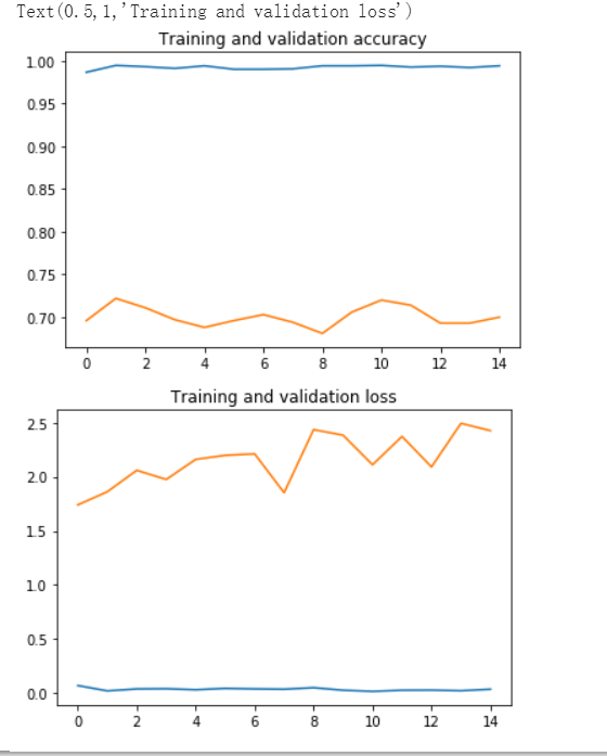
正如你所看到的，我们过度拟合就像它已经过时了。我们的训练准确度（蓝色）接近100％（！），而我们的验证准确度（绿色）停滞为70％。我们的验证损失在仅仅五个时期后达到最小值。

由于我们的培训实例数量相对较少（2000年），因此过度拟合应成为我们的首要关注点。过拟合发生在暴露于过几个例子，一个模型获悉不要推广到新的数据，模型开始使用不相关特征进行预测时，即模式。例如，如果你作为人类，只能看到三个伐木工人的图像，以及三个水手人的图像，其中唯一一个戴帽子的人是伐木工人，你可能会开始认为戴着帽子是一名伐木工人而不是水手的标志。然后你会做一个非常糟糕的伐木工人/水手分类器。

过度拟合是机器学习的核心问题：假设我们将模型的参数拟合到给定的数据集，我们如何确保模型学习的表示适用于以前从未见过的数据？我们如何避免学习特定于培训数据的内容？

在下一个练习中，我们将研究防止猫与狗分类模型过度拟合的方法。

Clean Up

在运行下一个练习之前，运行以下单元格以终止内核并释放内存资源：

import os, signal
os.kill(os.getpid(), signal.SIGKILL)

最后

以上就是生动黑夜最近收集整理的关于二十分钟构建猫VS狗图像分类器Cat vs. Dog Image Classification的全部内容，更多相关二十分钟构建猫VS狗图像分类器Cat内容请搜索靠谱客的其他文章。