我是靠谱客的博主 专注水蜜桃,这篇文章主要介绍Keras Alexnet Cat and Dog卷积神经网络发展史:网络结构如下:网络结构代码 AlexNet.py训练代码 train.py数据预处理 datasetprocess.py工具包 utils.py预测 perdict.py,现在分享给大家,希望可以做个参考。
文章目录
- 卷积神经网络发展史:
- 网络结构如下:
- 网络结构代码 AlexNet.py
- 训练代码 train.py
- 数据预处理 datasetprocess.py
- 工具包 utils.py
- 预测 perdict.py
卷积神经网络发展史:
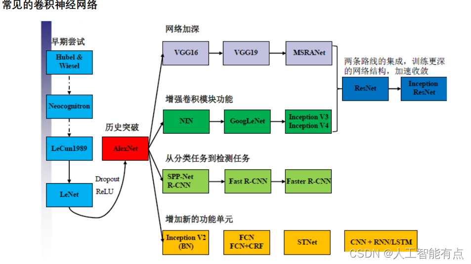
处理图像分类的经典神经网络-历史突破
网络结构如下:
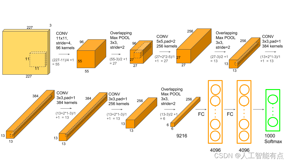
keras实现Alexnet + 猫狗分类
网络结构代码 AlexNet.py
from keras.models import Sequential
from keras.layers import Dense, Activation, Conv2D, MaxPooling2D, Flatten, Dropout, BatchNormalization
from keras.datasets import mnist
from keras.utils import np_utils
from keras.optimizers import Adam


# 注意,为了加快收敛,我将每个卷积层的filter减半,全连接层减为1024
def AlexNet(input_shape=(224, 224, 3), output_shape=2):
    # AlexNet 序贯模型
    model = Sequential()

    # 第一层卷积: 卷积激活 + 批标准化 + 池化
    # 使用步长为4x4,大小为11的卷积核对图像进行卷积,输出的特征层为96层,输出的shape为(55,55,96);
    # 所建模型后输出为48特征层
    model.add(
        Conv2D(
            filters=48,  # 48个卷积核(滤波器), 输出48个通道
            kernel_size=(11, 11),  # 卷积核大小(高宽)
            strides=(4, 4),  # 卷积核每次移动步长
            padding='valid',  # 填充方式使用valid
            input_shape=input_shape,  # 输入shape赋值
            activation='relu'  # 激活函数选择relu函数
        )
    )  # ->(55,55,48)
    # 批标准化
    model.add(BatchNormalization())
    # 使用步长为2的最大池化层进行池化,此时输出的shape为(27,27,96)
    # 所建模型后输出为48特征层
    model.add(
        MaxPooling2D(
            pool_size=(3, 3),
            strides=(2, 2),
            padding='valid'
        )
    )  # ->(27,27,48)

    # 第二层卷积: 卷积激活 + 批标准化 + 池化
    # 使用步长为1x1,大小为5的卷积核对图像进行卷积,输出的特征层为256层,输出的shape为(27,27,256);
    # 所建模型后输出为128特征层
    model.add(
        Conv2D(
            filters=128,
            kernel_size=(5, 5),
            strides=(1, 1),
            padding='same',
            activation='relu'
        )
    )  # ->(27,27,128)
    model.add(BatchNormalization())
    # 使用步长为2的最大池化层进行池化,此时输出的shape为(13,13,256);
    # 所建模型后输出为128特征层
    model.add(
        MaxPooling2D(
            pool_size=(3, 3),
            strides=(2, 2),
            padding='valid'
        )
    )  # ->(13,13,128)

    # 第三层卷积: 卷积激活
    # 使用步长为1x1,大小为3的卷积核对图像进行卷积,输出的特征层为384层,输出的shape为(13,13,384);
    # 所建模型后输出为192特征层
    model.add(
        Conv2D(
            filters=192,
            kernel_size=(3, 3),
            strides=(1, 1),
            padding='same',
            activation='relu'
        )
    )  # ->(13,13,192)

    # 第四层卷积: 卷积激活
    # 使用步长为1x1,大小为3的卷积核对图像进行卷积,输出的特征层为384层,输出的shape为(13,13,384);
    # 所建模型后输出为192特征层
    model.add(
        Conv2D(
            filters=192,
            kernel_size=(3, 3),
            strides=(1, 1),
            padding='same',
            activation='relu'
        )
    )  # ->(13,13,192)

    # 第五层卷积: 卷积激活 + 池化
    # 使用步长为1x1,大小为3的卷积核对图像进行卷积,输出的特征层为256层,输出的shape为(13,13,256);
    # 所建模型后输出为128特征层
    model.add(
        Conv2D(
            filters=128,
            kernel_size=(3, 3),
            strides=(1, 1),
            padding='same',
            activation='relu'
        )
    )  # ->(13,13,128)
    # 使用步长为2的最大池化层进行池化,此时输出的shape为(6,6,256);
    # 所建模型后输出为128特征层
    model.add(
        MaxPooling2D(
            pool_size=(3, 3),
            strides=(2, 2),
            padding='valid'
        )
    )  # ->(6,6,128)

    # 拍扁,变成一维
    model.add(Flatten())  # ->(4608 == 66*6*128)

    # 两个全连接层,最后输出为1000类,这里改为2类(猫和狗)
    # 缩减为1024
    # 第一个全连接层
    model.add(Dense(1024, activation='relu'))
    model.add(Dropout(0.25))

    # 第二个全连接层
    model.add(Dense(1024, activation='relu'))
    model.add(Dropout(0.25))

    # 第三个全连接层
    model.add(Dense(output_shape, activation='softmax'))

    return model
类似项目的深度学习的代码,是差不多的,区别是网络的不同。因此重构项目代码,只需要把模型结构重写即可。
训练代码 train.py
from keras.callbacks import TensorBoard, ModelCheckpoint, ReduceLROnPlateau, EarlyStopping
from keras.utils import np_utils
from keras.optimizers import Adam
import numpy as np
import utils
import cv2
from keras import backend as K

from model.AlexNet import AlexNet

# K.set_image_dim_ordering('tf')
# K.image_data_format() == 'channels_first'
# print(K.image_data_format())

def generate_arrays_from_file(lines, batch_size):
    # 获取总长度
    n = len(lines)
    i = 0
    while 1:
        X_train = []
        Y_train = []
        # 一个for循环获取一个batch_size大小的数据
        for b in range(batch_size):
            if i == 0:
                np.random.shuffle(lines)
            name = lines[i].split(';')[0]  # 文件名
            # 从文件中读取图像
            img = cv2.imread(r".dataimagetrain" + '/' + name)
            img = cv2.cvtColor(img, cv2.COLOR_BGR2RGB)
            img = img / 255  # 归一化
            X_train.append(img)
            Y_train.append(lines[i].split(';')[1])  # 标签
            # 读完一个周期后重新开始
            i = (i + 1) % n
        # 处理图像
        X_train = utils.resize_image(X_train, (224, 224))
        X_train = X_train.reshape(-1, 224, 224, 3)
        Y_train = np_utils.to_categorical(np.array(Y_train), num_classes=2)
        # yield 退出函数,下次调用接着执行,达到分批目的,节省内存
        yield (X_train, Y_train)


if __name__ == "__main__":
    # 模型保存的位置
    log_dir = "./logs/"

    # 打开数据集的txt
    with open(r".datadataset.txt", "r") as f:
        lines = f.readlines()

    # 打乱行,这个txt主要用于帮助读取数据来训练
    # 打乱的数据更有利于训练
    np.random.seed(10101)
    np.random.shuffle(lines)
    np.random.seed(None)

    # 90%用于训练,10%用于估计。
    num_val = int(len(lines) * 0.1)
    num_train = len(lines) - num_val

    # 建立AlexNet网络模型
    model = AlexNet()

    # 保存的方式,3代保存一次
    # 该回调函数将在每个epoch后保存模型到filepath
    checkpoint_period1 = ModelCheckpoint(
        log_dir + 'ep{epoch:03d}-loss{loss:.3f}-val_loss{val_loss:.3f}.h5',
        verbose=0,
        monitor='acc',
        mode='auto',
        save_weights_only=True,
        save_best_only=False,
        period=3
    )
    # 学习率下降的方式,acc三次不下降就下降学习率继续训练
    reduce_lr = ReduceLROnPlateau(
        monitor='acc',  # accuracy
        factor=0.5,
        patience=3,
        verbose=1
    )
    # 是否需要早停,当val_loss一直不下降的时候意味着模型基本训练完毕,可以停止
    early_stopping = EarlyStopping(
        monitor='val_loss',
        # min_delta=0,
        patience=10,
        verbose=1
    )

    # 交叉熵
    model.compile(
        loss='categorical_crossentropy',
        optimizer=Adam(lr=1e-3),
        metrics=['accuracy']
    )

    # 一次的训练集大小
    batch_size = 128

    print('Train on {} samples, val on {} samples, with batch size {}.'.format(num_train, num_val, batch_size))

    # 开始训练
    model.fit_generator(
        generator=generate_arrays_from_file(lines[:num_train], batch_size),
        steps_per_epoch=max(1, num_train // batch_size),
        validation_data=generate_arrays_from_file(lines[num_train:], batch_size),
        validation_steps=max(1, num_val // batch_size),
        epochs=50,
        initial_epoch=0,
        callbacks=[checkpoint_period1, reduce_lr, early_stopping])

    # 保存模型权重
    model.save_weights(log_dir + 'last2.h5')
数据预处理 datasetprocess.py
作用:把文件名和标签以字符串方式存在.txt文件中,在train.py中会用到这个.txt文件,读取data和label。
import os

photos = os.listdir("./data/image/train/")

# print(photos[:5])  # ['cat.0.jpg', 'cat.1.jpg', 'cat.10.jpg', 'cat.100.jpg', 'cat.1000.jpg']
with open("data/dataset.txt", "w") as f:
    for photoFileName in photos:
        name = photoFileName.split(".")[0]
        if name == "cat":
            f.write(photoFileName + ";0n")
        elif name == "dog":
            f.write(photoFileName + ";1n")
f.close()
工具包 utils.py
为perdict.py准备
import matplotlib.image as mpimg
import numpy as np
import cv2
import tensorflow as tf
from tensorflow.python.ops import array_ops


def load_image(path):
    # 读取图片,rgb
    img = mpimg.imread(path)
    # 将图片修剪成中心的正方形
    short_edge = min(img.shape[:2])
    yy = int((img.shape[0] - short_edge) / 2)
    xx = int((img.shape[1] - short_edge) / 2)
    crop_img = img[yy: yy + short_edge, xx: xx + short_edge]
    return crop_img


def resize_image(image, size):
    with tf.name_scope('resize_image'):
        images = []
        for i in image:
            i = cv2.resize(i, size)
            images.append(i)
        images = np.array(images)
        return images


def print_answer(argmax):
    with open("./data/model/index_word.txt", "r", encoding='utf-8') as f:
        synset = [l.split(";")[1][:-1] for l in f.readlines()]
    # print(synset[argmax])
    return synset[argmax]

#
# with open("./data/model/index_word.txt", "r", encoding='utf-8') as f:
#     # synset = [l.split(";")[1][:-1] for l in f.readlines()]
#     # print(synset)
#     for l in f.readlines():
#         print(l.split(';')[1][:-1])
预测 perdict.py
import numpy as np
import utils
import cv2
from keras import backend as K
from model.AlexNet import AlexNet

# K.set_image_dim_ordering('tf')
# K.image_data_format() == 'channels_first'

if __name__ == "__main__":
    model = AlexNet()
    model.load_weights("./logs/last1.h5")
    img = cv2.imread("./test4.jpg")
    img_RGB = cv2.cvtColor(img, cv2.COLOR_BGR2RGB)
    img_nor = img_RGB / 255
    img_nor = np.expand_dims(img_nor, axis=0)  # 增加维度
    img_resize = utils.resize_image(img_nor, (224, 224))
    print('the answer is: ', utils.print_answer(np.argmax(model.predict(img_resize))))
    cv2.imshow("ooo", img)
    cv2.waitKey(0)
read("./test4.jpg")
    img_RGB = cv2.cvtColor(img, cv2.COLOR_BGR2RGB)
    img_nor = img_RGB / 255
    img_nor = np.expand_dims(img_nor, axis=0)  # 增加维度
    img_resize = utils.resize_image(img_nor, (224, 224))
    print('the answer is: ', utils.print_answer(np.argmax(model.predict(img_resize))))
    cv2.imshow("ooo", img)
    cv2.waitKey(0)
最后
以上就是专注水蜜桃最近收集整理的关于Keras Alexnet Cat and Dog卷积神经网络发展史:网络结构如下:网络结构代码 AlexNet.py训练代码 train.py数据预处理 datasetprocess.py工具包 utils.py预测 perdict.py的全部内容,更多相关Keras内容请搜索靠谱客的其他文章。
本图文内容来源于网友提供,作为学习参考使用,或来自网络收集整理,版权属于原作者所有。


发表评论 取消回复