cs231n的第一次作业svm

SVM算dw

svm实现公式中,线性函数为

损失函数为

为了更快得到期望W，需要找寻梯度dw。图像数据Xi = [ D*1 ]，W[k*D]或者W[k*D+1]，k表示有k个类别。W的每一个行向量便是一个分类器。

对某个数据点上的损失计算

即 Li = （Wj行对Xi的分数 - Wyi行对Xi分类正确的分数 + delta）

如果Li小于0，则Li = 0。对其求Wyi的偏导数和Wj的偏导数，结果分别为 -Xi和Xi（如果Li大于0的话，否则偏导为0）。所以在计算损失的同时，可以更新偏导数dw。这就是这几句程序的意思：

if margin > 0:
    loss += margin

    dW[:, j] += X[i].T
    dW[:, y[i]] -= X[i].T

感觉好像有一个问题，对一个矩阵的转置求导数是什么？

这样子？

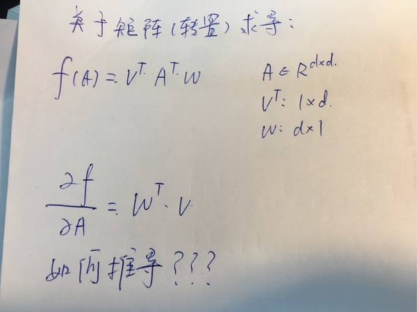
整体代码如下：

def svm_loss_naive(W, X, y, reg):
  """
  Structured SVM loss function, naive implementation (with loops).

  Inputs have dimension D, there are C classes, and we operate on minibatches of N examples.

  Inputs:
  - W: A numpy array of shape (D, C) containing weights.
  - X: A numpy array of shape (N, D) containing a minibatch of data.
  - y: A numpy array of shape (N,) containing training labels; y[i] = c means
    that X[i] has label c, where 0 <= c < C.
  - reg: (float) regularization strength

  Returns a tuple of:
  - loss as single float
  - gradient with respect to weights W; an array of same shape as W
  """
  dW = np.zeros(W.shape) # initialize the gradient as zero

  # compute the loss and the gradient
  num_classes = W.shape[1]
  num_train = X.shape[0]
  loss = 0.0
  for i in xrange(num_train):
    scores = X[i].dot(W)
    correct_class_score = scores[y[i]]
    for j in xrange(num_classes):
      if j == y[i]:
        continue
      margin = scores[j] - correct_class_score + 1 # note delta = 1
      if margin > 0:
        loss += margin

        dW[:, j] += X[i].T
        dW[:, y[i]] -= X[i].T

  loss /= num_train
  dW /= num_train

  # Add regularization to the loss.
  loss += 0.5 * reg * np.sum(W * W)
  dW += reg * W

  return loss, dW

loss最后加了正则项
注意这里loss和dW都要除以num_train。否则样本越多，loss越大.

两种方法的所需时间和最后dw的差异：

Naive loss and gradient: computed in 0.103881s
Vectorized loss and gradient: computed in 0.003264s
difference: 0.000000

2.上述方法逐一对w进行微量变化，并求导数的方式步骤繁琐，并且产生了很多不必要的步骤。另外一种（矩阵）直接算loss和dw的方法

def svm_loss_vectorized(W, X, y, reg):
  """
  Structured SVM loss function, vectorized implementation.

  Inputs and outputs are the same as svm_loss_naive.
  """
  loss = 0.0
  dW = np.zeros(W.shape) # initialize the gradient as zero

  #pass
  scores = X.dot(W)  # N by C
  num_train = X.shape[0]
  scores_correct = scores[np.arange(num_train), y]  # 1 by N
  scores_correct = np.reshape(scores_correct, (num_train, 1))  # N by 1
  margins = scores - scores_correct + 1.0  # N by C
  margins[np.arange(num_train), y] = 0.0
  margins[margins <= 0] = 0.0
  loss += np.sum(margins) / num_train
  loss += 0.5 * reg * np.sum(W * W)

  margins[margins > 0] = 1.0
  row_sum = np.sum(margins, axis=1)  # 1 by N
  margins[np.arange(num_train), y] = -row_sum
  dW += np.dot(X.T, margins) / num_train + reg * W  # D by C
  return loss, dW

对于loss，间隔margins中把j=yi项赋值为0，margins小于0处赋值为0，对剩下的元素求和取平均，最后加上正则项。
对于dw，首先间隔margins小于0处赋值为0，其余赋值为1。dWj = X.T.dot(margins)。对应的dWyi = -X.T.dot(margins)。

验证算得的loss和dw的正确性

from cs231n.gradient_check import grad_check_sparse

grad_check_sparse利用中心差值公式[f(x+h) - f(x-h)] / 2h 计算梯度。
这里没有用中心差值，只是个小例子，方便理解。

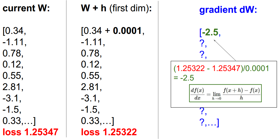
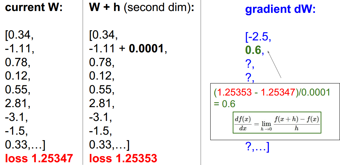
算f(x)的时候还是用到了svm_loss_naive，返回的第一个参数便是loss
当然最后dw的结果会有差异，因为h只是象征性的取了一个极小值。

用随机梯度下降(Stochastic Gradient Descent，SGD)来最小化loss

考虑到训练数据X庞大，为了一个参数的更新而计算整个训练集太浪费了。一个常用的方法是计算训练集中的小批量数据（相当于样本n，有点类似）。X_batch 和 y_batch 即每次选的小批数据来更新权重W。下面函数将每次更新完的loss保存在数组loss_hist中，方便画图看不同迭代次数后的loss。

  def train(self, X, y, learning_rate=1e-3, reg=1e-5, num_iters=100,
            batch_size=200, verbose=False):
    """
    Train this linear classifier using stochastic gradient descent.

    Inputs:
    - X: A numpy array of shape (N, D) containing training data; there are N
      training samples each of dimension D.
    - y: A numpy array of shape (N,) containing training labels; y[i] = c means that X[i] has label 0 <= c < C for C classes.
    - learning_rate: (float) learning rate for optimization.
    - reg: (float) regularization strength.
    - num_iters: (integer) number of steps to take when optimizing
    - batch_size: (integer) number of training examples to use at each step.
    - verbose: (boolean) If true, print progress during optimization.

    Outputs:
    A list containing the value of the loss function at each training iteration.
    """
    num_train, dim = X.shape
    num_classes = np.max(y) + 1 # assume y takes values 0...K-1 where K is number of classes
    if self.W is None:
      # lazily initialize W
      self.W = 0.001 * np.random.randn(dim, num_classes)

    # Run stochastic gradient descent to optimize W
    loss_history = []
    for it in xrange(num_iters):
      X_batch = None
      y_batch = None

      sample_index = np.random.choice(num_train, batch_size, replace=False)
      X_batch = X[sample_index, :]  # batch_size by D
      y_batch = y[sample_index]  # 1 by batch_size

      # evaluate loss and gradient
      loss, grad = self.loss(X_batch, y_batch, reg)
      loss_history.append(loss)


      self.W -= learning_rate * grad



      if verbose and it % 100 == 0:
        print 'iteration %d / %d: loss %f' % (it, num_iters, loss)

    return loss_history

plt.plot(loss_hist)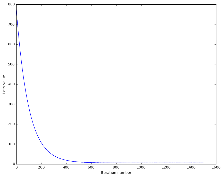

迭代500次后loss基本稳定。

最后预测

  def predict(self, X):
    """
    Use the trained weights of this linear classifier to predict labels for data points.
    Inputs:
    - X: D x N array of training data. Each column is a D-dimensional point.

    Returns:
    - y_pred: Predicted labels for the data in X. y_pred is a 1-dimensional array of length N, and each element is an integer giving the predicted class.
    """
    y_pred = np.zeros(X.shape[1])

    print self.W.shape,X.shape
    score = np.dot(X,self.W)
    print score.shape
    y_pred = np.argmax(score, axis=1)

    print y_pred.shape
    return y_pred

training accuracy: 0.363857
validation accuracy: 0.373000

2.测试集正确率为37.3%，相比训练集的准确率而言提高了，泛化性能可以啊。图片线性程度不高，可能是正确率较低的原因。

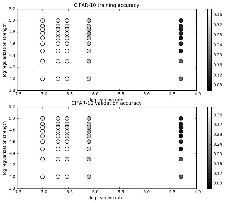
最后对学习率和正则化强度这两个超参数进行训练，选取较好的参数。

learning_rates = [1e-7, 2e-7, 3e-7, 5e-5, 8e-7]
regularization_strengths = [1e4, 2e4, 3e4, 4e4, 5e4, 6e4, 7e4, 8e4, 1e5]

# results is dictionary mapping tuples of the form
# (learning_rate, regularization_strength) to tuples of the form
# (training_accuracy, validation_accuracy). The accuracy is simply the fraction
# of data points that are correctly classified.
results = {}
best_val = -1   # The highest validation accuracy that we have seen so far.
best_svm = None # The LinearSVM object that achieved the highest validation rate.

iters = 1500 
for lr in learning_rates:    
    for rs in regularization_strengths:
        svm = LinearSVM()
        svm.train(X_train, y_train, learning_rate=lr, reg=rs, num_iters=iters)
        y_train_pred = svm.predict(X_train)
        accu_train = np.mean(y_train == y_train_pred)
        y_val_pred = svm.predict(X_val)
        accu_val = np.mean(y_val == y_val_pred)

        results[(lr, rs)] = (accu_train, accu_val)

        if best_val < accu_val:
            best_val = accu_val
            best_svm = svm

# Print out results.
for lr, reg in sorted(results):
    train_accuracy, val_accuracy = results[(lr, reg)]
    print 'lr %e reg %e train accuracy: %f val accuracy: %f' % (
                lr, reg, train_accuracy, val_accuracy)

print 'best validation accuracy achieved during cross-validation: %f' % best_val

1.跑了n久后，至少分钟计（学习率和正则化强度取值太多了。。），得到结果

lr 1.000000e-07 reg 1.000000e+04 train accuracy: 0.377245 val accuracy: 0.394000
lr 1.000000e-07 reg 2.000000e+04 train accuracy: 0.383469 val accuracy: 0.381000
lr 1.000000e-07 reg 3.000000e+04 train accuracy: 0.372959 val accuracy: 0.390000
lr 1.000000e-07 reg 4.000000e+04 train accuracy: 0.375571 val accuracy: 0.392000
lr 1.000000e-07 reg 5.000000e+04 train accuracy: 0.369959 val accuracy: 0.386000
lr 1.000000e-07 reg 6.000000e+04 train accuracy: 0.369857 val accuracy: 0.387000
lr 1.000000e-07 reg 7.000000e+04 train accuracy: 0.360204 val accuracy: 0.377000
lr 1.000000e-07 reg 8.000000e+04 train accuracy: 0.361469 val accuracy: 0.374000
lr 1.000000e-07 reg 1.000000e+05 train accuracy: 0.351163 val accuracy: 0.353000
lr 2.000000e-07 reg 1.000000e+04 train accuracy: 0.383245 val accuracy: 0.384000
lr 2.000000e-07 reg 2.000000e+04 train accuracy: 0.373306 val accuracy: 0.379000
lr 2.000000e-07 reg 3.000000e+04 train accuracy: 0.371184 val accuracy: 0.386000
lr 2.000000e-07 reg 4.000000e+04 train accuracy: 0.370694 val accuracy: 0.363000
lr 2.000000e-07 reg 5.000000e+04 train accuracy: 0.354102 val accuracy: 0.371000
lr 2.000000e-07 reg 6.000000e+04 train accuracy: 0.362633 val accuracy: 0.363000
lr 2.000000e-07 reg 7.000000e+04 train accuracy: 0.350918 val accuracy: 0.365000
lr 2.000000e-07 reg 8.000000e+04 train accuracy: 0.354449 val accuracy: 0.351000
lr 2.000000e-07 reg 1.000000e+05 train accuracy: 0.344122 val accuracy: 0.353000
lr 3.000000e-07 reg 1.000000e+04 train accuracy: 0.373490 val accuracy: 0.390000
lr 3.000000e-07 reg 2.000000e+04 train accuracy: 0.360857 val accuracy: 0.357000
lr 3.000000e-07 reg 3.000000e+04 train accuracy: 0.372816 val accuracy: 0.394000
lr 3.000000e-07 reg 4.000000e+04 train accuracy: 0.357510 val accuracy: 0.365000
lr 3.000000e-07 reg 5.000000e+04 train accuracy: 0.354102 val accuracy: 0.347000
lr 3.000000e-07 reg 6.000000e+04 train accuracy: 0.359633 val accuracy: 0.365000
lr 3.000000e-07 reg 7.000000e+04 train accuracy: 0.350510 val accuracy: 0.353000
lr 3.000000e-07 reg 8.000000e+04 train accuracy: 0.349061 val accuracy: 0.344000
lr 3.000000e-07 reg 1.000000e+05 train accuracy: 0.346612 val accuracy: 0.354000
lr 8.000000e-07 reg 1.000000e+04 train accuracy: 0.339265 val accuracy: 0.321000
lr 8.000000e-07 reg 2.000000e+04 train accuracy: 0.296959 val accuracy: 0.305000
lr 8.000000e-07 reg 3.000000e+04 train accuracy: 0.343694 val accuracy: 0.352000
lr 8.000000e-07 reg 4.000000e+04 train accuracy: 0.307837 val accuracy: 0.305000
lr 8.000000e-07 reg 5.000000e+04 train accuracy: 0.308224 val accuracy: 0.328000
lr 8.000000e-07 reg 6.000000e+04 train accuracy: 0.267980 val accuracy: 0.278000
lr 8.000000e-07 reg 7.000000e+04 train accuracy: 0.283408 val accuracy: 0.296000
lr 8.000000e-07 reg 8.000000e+04 train accuracy: 0.310388 val accuracy: 0.318000
lr 8.000000e-07 reg 1.000000e+05 train accuracy: 0.292633 val accuracy: 0.293000
lr 5.000000e-05 reg 1.000000e+04 train accuracy: 0.197327 val accuracy: 0.180000
lr 5.000000e-05 reg 2.000000e+04 train accuracy: 0.178531 val accuracy: 0.170000
lr 5.000000e-05 reg 3.000000e+04 train accuracy: 0.089224 val accuracy: 0.075000
lr 5.000000e-05 reg 4.000000e+04 train accuracy: 0.104633 val accuracy: 0.105000
lr 5.000000e-05 reg 5.000000e+04 train accuracy: 0.058898 val accuracy: 0.059000
lr 5.000000e-05 reg 6.000000e+04 train accuracy: 0.100265 val accuracy: 0.087000
lr 5.000000e-05 reg 7.000000e+04 train accuracy: 0.100265 val accuracy: 0.087000
lr 5.000000e-05 reg 8.000000e+04 train accuracy: 0.100265 val accuracy: 0.087000
lr 5.000000e-05 reg 1.000000e+05 train accuracy: 0.100265 val accuracy: 0.087000
best validation accuracy achieved during cross-validation: 0.394000
1.正确率到了39.4%，提高了一点
2.还是图标比较实在

lr 3.000000e-07 reg 3.000000e+04用这组在训练集上表现最好的超参数来对测试集测试

linear SVM on raw pixels final test set accuracy: 0.374000
相比与之前的37.3%.提高了0.1%，，，(⊙o⊙)…

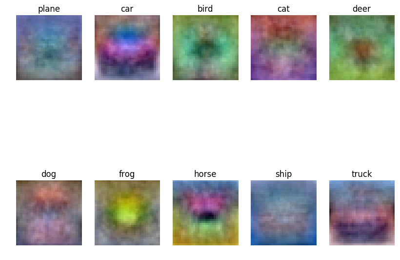
最后来看看模板W长啥样吧

小结

f = Wx
dw = x
dw只与数据有关，而与权重W无关

参考

知乎翻译赞https://zhuanlan.zhihu.com/p/21360434?refer=intelligentunit
http://www.cnblogs.com/wangxiu/p/5668659.html
http://www.cnblogs.com/wangxiu/p/5514765.html

最后

以上就是拼搏奇迹为你收集整理的cs231n的第一次作业svm的全部内容，希望文章能够帮你解决cs231n的第一次作业svm所遇到的程序开发问题。

如果觉得靠谱客网站的内容还不错，欢迎将靠谱客网站推荐给程序员好友。