此示例显示如何为强化学习策略定义自定义训练循环。 您可以使用此工作流程通过您自己的自定义训练算法来训练强化学习策略，而不是使用Reinforcement Learning Toolbox™软件中的内置智能体之一。

使用此工作流程，您可以训练使用以下任何策略和值函数表示形式的策略。

1. rlStochasticActorRepresentation —随机行动者表示

2. rlDeterministicActorRepresentation —确定性行动者表示

3. rlValueRepresentation —值函数评论者表示

4. rlQValueRepresentation — Q值函数评论者表示

在此示例中，使用REINFORCE算法（没有基线）来训练具有离散操作空间的随机行动者策略。 有关REINFORCE算法的更多信息，请参阅策略梯度智能体。

固定随机生成器种子的再现性。

rng(0)

有关可用于自定义训练的功能的更多信息，请参阅自定义训练的功能。

环境

对于此示例，强化学习策略是在离散的倒立摆环境中训练的。 在这种环境下的目标是通过在推车上施加力（作用）来平衡杆。 使用rlPredefinedEnv函数创建环境。

env = rlPredefinedEnv('CartPole-Discrete');

从环境中提取观察和行动规范。

obsInfo = getObservationInfo(env);
actInfo = getActionInfo(env);

获取观察数（numObs）和动作数（numAct）。

numObs = obsInfo.Dimension(1);
numAct = actInfo.Dimension(1);

策略

在此示例中，强化学习策略是离散动作随机策略。 它由一个深度神经网络表示，该网络包含fullyConnectedLayer，reluLayer和softmaxLayer层。 给定当前观测值，该网络输出每个离散动作的概率。 softmaxLayer可以确保表示形式输出的概率值范围为[0 1]，并且所有概率之和为1。

为行动者创建深度神经网络。

actorNetwork = [featureInputLayer(numObs,'Normalization','none','Name','state')
                fullyConnectedLayer(24,'Name','fc1')
                reluLayer('Name','relu1')
                fullyConnectedLayer(24,'Name','fc2')
                reluLayer('Name','relu2')
                fullyConnectedLayer(2,'Name','output')
                softmaxLayer('Name','actionProb')];

使用rlStochasticActorRepresentation对象创建行动者表示。

actorOpts = rlRepresentationOptions('LearnRate',1e-3,'GradientThreshold',1);
actor = rlStochasticActorRepresentation(actorNetwork,...
    obsInfo,actInfo,'Observation','state',actorOpts);

对于此示例，该策略的损失函数在actorLossFunction中实现。

使用setLoss函数设置损失函数。

actor = setLoss(actor,@actorLossFunction);

训练设置

配置训练以使用以下选项：

1. 将训练设置为最多持续5000个episode ，每个episode 最多持续250个步骤。

2. 要计算折扣奖励，请选择0.995的折扣系数。

3. 在达到最大episode 次数后或在100个episode 中的平均奖励达到220的值时终止训练。

numEpisodes = 5000;
maxStepsPerEpisode = 250;
discountFactor = 0.995;
aveWindowSize = 100;
trainingTerminationValue = 220;

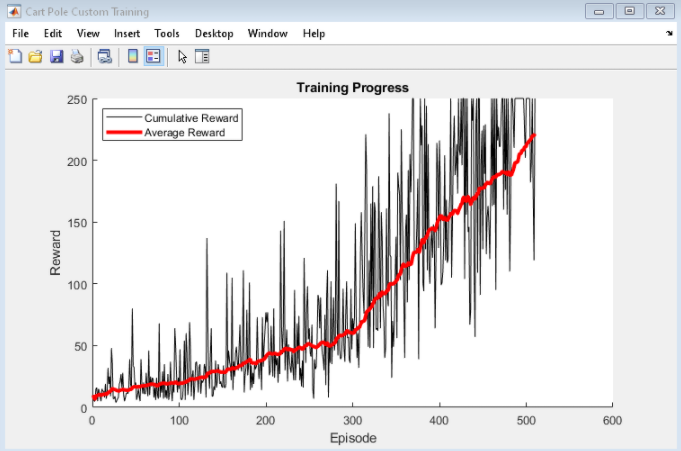
创建一个向量来存储每个训练episode 的累积奖励。

episodeCumulativeRewardVector = [];

使用hBuildFigure辅助函数创建用于训练可视化的图形。

[trainingPlot,lineReward,lineAveReward] = hBuildFigure;

自定义训练循环

自定义训练循环的算法如下。 对于每个episode：

1. 重置环境。

2. 创建用于存储经验信息的缓冲区：观察，动作和奖励。

3. 产生经验，直到最终情况发生。 为此，请评估策略以采取措施，将这些措施应用于环境，并获得最终的观察结果和回报。 将动作，观察结果和奖励存储在缓冲区中。

4. 收集训练数据作为一批经验。

5. 计算episode蒙特卡洛的收益，这是折扣的未来奖励。

6. 根据策略表示参数计算损失函数的梯度。

7. 使用计算出的梯度来更新行动者表示。

8. 更新训练可视化。

9. 如果对策略进行了充分的训练，请终止训练。

% Enable the training visualization plot.
set(trainingPlot,'Visible','on');

% Train the policy for the maximum number of episodes or until the average
% reward indicates that the policy is sufficiently trained.
for episodeCt = 1:numEpisodes
    
    % 1. Reset the environment at the start of the episode
    obs = reset(env);
    
    episodeReward = zeros(maxStepsPerEpisode,1);
    
    % 2. Create buffers to store experiences. The dimensions for each buffer
    % must be as follows.
    %
    % For observation buffer: 
    %     numberOfObservations x numberOfObservationChannels x batchSize
    %
    % For action buffer: 
    %     numberOfActions x numberOfActionChannels x batchSize
    %
    % For reward buffer: 
    %     1 x batchSize
    %
    observationBuffer = zeros(numObs,1,maxStepsPerEpisode);
    actionBuffer = zeros(numAct,1,maxStepsPerEpisode);
    rewardBuffer = zeros(1,maxStepsPerEpisode);
    
    % 3. Generate experiences for the maximum number of steps per
    % episode or until a terminal condition is reached.
    for stepCt = 1:maxStepsPerEpisode
        
        % Compute an action using the policy based on the current 
        % observation.
        action = getAction(actor,{obs});
        
        % Apply the action to the environment and obtain the resulting
        % observation and reward.
        [nextObs,reward,isdone] = step(env,action{1});
        
        % Store the action, observation, and reward experiences in buffers.
        observationBuffer(:,:,stepCt) = obs;
        actionBuffer(:,:,stepCt) = action{1};
        rewardBuffer(:,stepCt) = reward;
        
        episodeReward(stepCt) = reward;
        obs = nextObs;
        
        % Stop if a terminal condition is reached.
        if isdone
            break;
        end
        
    end
    
    % 4. Create training data. Training is performed using batch data. The
    % batch size equal to the length of the episode.
    batchSize = min(stepCt,maxStepsPerEpisode);
    observationBatch = observationBuffer(:,:,1:batchSize);
    actionBatch = actionBuffer(:,:,1:batchSize);
    rewardBatch = rewardBuffer(:,1:batchSize);

    % Compute the discounted future reward.
    discountedReturn = zeros(1,batchSize);
    for t = 1:batchSize
        G = 0;
        for k = t:batchSize
            G = G + discountFactor ^ (k-t) * rewardBatch(k);
        end
        discountedReturn(t) = G;
    end

    % 5. Organize data to pass to the loss function.
    lossData.batchSize = batchSize;
    lossData.actInfo = actInfo;
    lossData.actionBatch = actionBatch;
    lossData.discountedReturn = discountedReturn;
    
    % 6. Compute the gradient of the loss with respect to the policy
    % parameters.
    actorGradient = gradient(actor,'loss-parameters',...
        {observationBatch},lossData);
    
    % 7. Update the actor network using the computed gradients.
    actor = optimize(actor,actorGradient);

    % 8. Update the training visualization.
    episodeCumulativeReward = sum(episodeReward);
    episodeCumulativeRewardVector = cat(2,...
        episodeCumulativeRewardVector,episodeCumulativeReward);
    movingAveReward = movmean(episodeCumulativeRewardVector,...
        aveWindowSize,2);
    addpoints(lineReward,episodeCt,episodeCumulativeReward);
    addpoints(lineAveReward,episodeCt,movingAveReward(end));
    drawnow;
    
    % 9. Terminate training if the network is sufficiently trained.
    if max(movingAveReward) > trainingTerminationValue
        break
    end
    
end

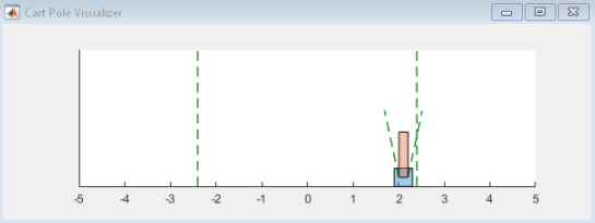
仿真

训练结束后，模拟训练策略。

在模拟之前，请重置环境。

obs = reset(env);

启用环境可视化，该环境可视化在每次调用环境步骤函数时更新。

plot(env)

对于每个模拟步骤，请执行以下操作。

1. 使用getAction函数从策略中采样以获取操作。

2. 使用获得的动作值逐步执行环境。

3. 如果达到终止条件，则终止。

for stepCt = 1:maxStepsPerEpisode
    
    % Select action according to trained policy
    action = getAction(actor,{obs});
        
    % Step the environment
    [nextObs,reward,isdone] = step(env,action{1});
    
    % Check for terminal condition
    if isdone
        break
    end
    
    obs = nextObs;
    
end

自定义训练函数

要从“强化学习工具箱”策略和值函数表示中获取给定观察值的动作和值函数，可以使用以下函数。

1. getValue —获得估计的状态值或状态作用值函数。

2. getAction —根据当前观察值从行动者表示中获取动作。

3. getMaxQValue —获取离散Q值表示形式的估计最大状态作用值函数。

如果您的策略或价值函数表示是循环神经网络，即具有至少一层具有隐藏状态信息的神经网络，则前面的函数可以返回当前网络状态。 您可以使用以下函数语法来获取和设置表示形式的状态。

1. state = getState（rep）—获取表示形式rep的状态。

2. newRep = setState（oldRep，state）—设置表示形式oldRep的状态，并在oldRep中返回结果。

3. newRep = resetState（oldRep）—将oldRep的所有状态值重置为零，并在newRep中返回结果。

您可以分别使用getLearnableParameters和setLearnableParameters函数获取和设置表示形式的可学习参数。

除了这些功能之外，您还可以使用setLoss，gradient，optimize和syncParameters函数来设置参数并计算策略和值函数表示形式的梯度。

setLoss

以随机梯度上升的方式训练策略，其中使用损失函数的梯度来更新网络。 对于自定义训练，您可以使用setLoss函数设置损失函数。 为此，请使用以下语法。

newRep = setLoss(oldRep,lossFcn)

这里：

1. oldRep是策略或值函数表示对象。

2. lossFcn是自定义损失函数的名称或自定义损失函数的句柄。

3. newRep与oldRep等效，只是将损失函数添加到表示中。

gradient

梯度函数计算表示损失函数的梯度。 您可以计算几个不同的梯度。 例如，要计算表示形式输出相对于其输入的梯度，请使用以下语法。

grad = gradient(rep,“output-input”,inputData)

这里：

1. rep是策略或值函数表示对象。

2. inputData包含表示形式的输入通道的值。

3. grad包含计算出的梯度。

有关更多信息，请在MATLAB命令行中键入

help rl.representation.rlAbstractRepresentation.gradient.

optimize

优化函数基于计算的梯度更新表示的可学习参数。 要更新梯度参数，请使用以下语法。

newRep = optimize(oldRep,grad)

在这里，oldRep是策略或值函数表示对象，并且grad包含使用梯度函数计算的梯度。 newRep与oldRep具有相同的结构，但是其参数已更新。

syncParameters

syncParameters函数根据另一种表示形式的策略或值函数表示的可学习参数进行更新。 与DDPG智能体一样，此功能对于更新目标行动者或评论者表示很有用。 要在两个表示之间同步参数值，请使用以下语法。

newTargetRep = syncParameters(oldTargetRep,sourceRep,smoothFactor)

这里：

1. oldTargetRep是一个带有参数${\theta }_{old}$的策略或值函数表示对象。
2. sourceRep是一个策略或值函数表示对象，与oldTargetRep具有相同的结构，但参数是${\theta }_{source}$。
3. smoothFactor 是更新的光滑因子(τ)。
4. newTargetRep与oldRep具有相同的结构，但其参数为${\theta }_{new}=\tau {\theta }_{source}+(1-\tau ){\theta }_{old}$。

损失函数

REINFORCE算法中的损失函数是折扣奖励和策略对数的乘积，该乘积跨所有时间步进行求和。 必须调整在自定义训练循环中计算的折扣奖励的大小，以使其与乘数策略兼容。

function loss = actorLossFunction(policy, lossData)

    % Create the action indication matrix.
    batchSize = lossData.batchSize;
    Z = repmat(lossData.actInfo.Elements',1,batchSize);
    actionIndicationMatrix = lossData.actionBatch(:,:) == Z;
    
    % Resize the discounted return to the size of policy.
    G = actionIndicationMatrix .* lossData.discountedReturn;
    G = reshape(G,size(policy));
    
    % Round any policy values less than eps to eps.
    policy(policy < eps) = eps;
    
    % Compute the loss.
    loss = -sum(G .* log(policy),'all');
    
end

帮助函数

以下帮助函数创建了一个图形，用于训练可视化。

function [trainingPlot, lineReward, lineAveReward] = hBuildFigure()
    plotRatio = 16/9;
    trainingPlot = figure(...
                'Visible','off',...
                'HandleVisibility','off', ...
                'NumberTitle','off',...
                'Name','Cart Pole Custom Training');
    trainingPlot.Position(3) = plotRatio * trainingPlot.Position(4);
    
    ax = gca(trainingPlot);
    
    lineReward = animatedline(ax);
    lineAveReward = animatedline(ax,'Color','r','LineWidth',3);
    xlabel(ax,'Episode');
    ylabel(ax,'Reward');
    legend(ax,'Cumulative Reward','Average Reward','Location','northwest')
    title(ax,'Training Progress');
end

最后

以上就是辛勤方盒最近收集整理的关于MATLAB强化学习实战(十一) 使用自定义训练循环训练强化学习策略环境策略训练设置自定义训练循环仿真自定义训练函数损失函数帮助函数的全部内容，更多相关MATLAB强化学习实战(十一)内容请搜索靠谱客的其他文章。