已知微分方程或传递函数的PID控制器设计

103 阅读 0 评论 68 点赞

我是靠谱客的博主丰富萝莉，这篇文章主要介绍已知微分方程或传递函数的PID控制器设计，现在分享给大家，希望可以做个参考。

PID的理论工作比较成熟，在实际编程时可能会遇到问题，如果只是简单的二阶惯性系统（ $\overset{s}{¨} = u$ ），可以比较容易的求出输出，并且与输入做差，再进行一个PID控制。如果是一个 $\overset{s}{¨} = - s + \overset{s}{˙} + u$ ，可能就有同学不会算输出了。如果用matlab的Simulink的话，可以很简单的拖动框图来设计，比如上面的微分方程如果用Simulink设计一个PID控制器，总体的设计图如下：
PID控制器Simulink设计图
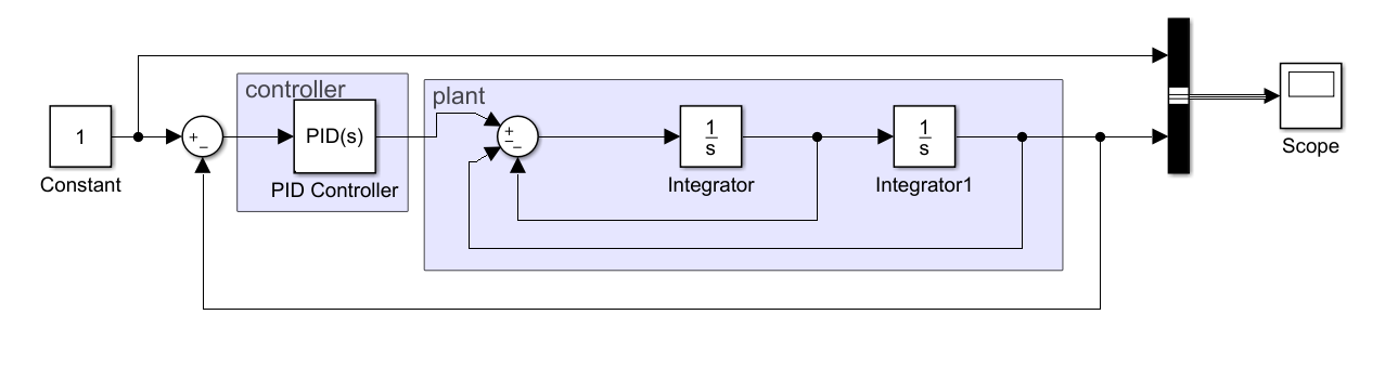
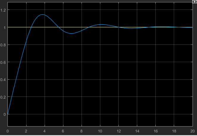
PID的参数选择Kp=0.5，Kd=1，Ki=0.5。仿真时间为20s，仿真图如下：
在这里插入图片描述
上面是用Simulink的方式设计PID，下面用写代码的方式来设计。在此，已知微分方程或者传递函数的情况下，把PID的控制器设计过程采用下面三种方法进行。
（1）ode解法
（2）欧拉法
（3）由Z域解得差分方程
已知一个系统的微分方程如下：
$\ y= x end{array} right.$
设控制目标为 $v = 1$ ，如何设计这个系统的PID控制器呢？
（1）ode解法
ode是matlab中用于计算微分方程数值解的工具，具体的介绍参考这篇博文【MATLAB】关于ode45的一部分用法，首先将被控对象写成两个一阶的微分方程：
$dot{x_1}=x_2=dot{x} & \ dot{x_2}=-x_1-x_2+u end{array} right.$
这个被控对象的matlab代码如下：

复制代码

1
2
3
4
5
6
7
8
function dx = ADRC1_1_4Plant(t,x,para)

u=para;

dx = zeros(2, 1);
dx(1) = x(2);
dx(2) = -x(1)-x(2)+u;

然后是主程序的代码：

复制代码

%Discrete PID control for continuous plant
clear all;
close all;
Kp = 0.5;
Ki = 1;
Kd = 0.5;

sampleTime = 0.01; %sample time
xInit=zeros(2,1);
e_1=0.0; %last time error
errorSum = 0.0; %the error integral
u_1 = 0; %initial control is 0

for k=1:1:2000
    time(k) = k*sampleTime;
    inputRef(k)=1; %step signal
    
    para=u_1;
    timeSpan=[0 sampleTime];
    [tCurrent,xCurrent]=ode45(@(t,x) ADRC1_1_4Plant(t,x,para),timeSpan,xInit);%get(t,x)
    xInit = xCurrent(length(xCurrent),:);%xInit as the next time begin
    y(k)=xInit(1);
    
    e(k)=inputRef(k)-y(k);
    errorSum = errorSum+e(k)*sampleTime;
    de(k)=(e(k)-e_1)/sampleTime;
    u(k)=Kp*e(k) + Ki*errorSum + Kd*de(k);
    %%Control limit
    if u(k)>10.0
        u(k)=10.0;
    end
    if u(k)<-10.0
        u(k)=-10.0;
    end
    u_1 = u(k);
    e_1 = e(k);
end

figure(1);
plot(time,inputRef,'r',time,y,'k:','linewidth',2);
xlabel('time(s)');ylabel('yd,y');
legend('Ideal position signal','Position tracking');
figure(2);
plot(time,inputRef-y,'r','linewidth',2);
xlabel('time(s)'),ylabel('error');

1
2
3
4
5
6
7
8
9
10
11
12
13
14
15
16
17
18
19
20
21
22
23
24
25
26
27
28
29
30
31
32
33
34
35
36
37
38
39
40
41
42
43
44
45
46
%Discrete PID control for continuous plant
clear all;
close all;
Kp = 0.5;
Ki = 1;
Kd = 0.5;

sampleTime = 0.01; %sample time
xInit=zeros(2,1);
e_1=0.0; %last time error
errorSum = 0.0; %the error integral
u_1 = 0; %initial control is 0

for k=1:1:2000
    time(k) = k*sampleTime;
    inputRef(k)=1; %step signal
    
    para=u_1;
    timeSpan=[0 sampleTime];
    [tCurrent,xCurrent]=ode45(@(t,x) ADRC1_1_4Plant(t,x,para),timeSpan,xInit);%get(t,x)
    xInit = xCurrent(length(xCurrent),:);%xInit as the next time begin
    y(k)=xInit(1);
    
    e(k)=inputRef(k)-y(k);
    errorSum = errorSum+e(k)*sampleTime;
    de(k)=(e(k)-e_1)/sampleTime;
    u(k)=Kp*e(k) + Ki*errorSum + Kd*de(k);
    %%Control limit
    if u(k)>10.0
        u(k)=10.0;
    end
    if u(k)<-10.0
        u(k)=-10.0;
    end
    u_1 = u(k);
    e_1 = e(k);
end

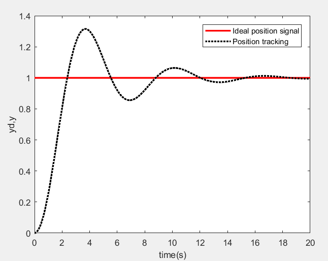
figure(1);
plot(time,inputRef,'r',time,y,'k:','linewidth',2);
xlabel('time(s)');ylabel('yd,y');
legend('Ideal position signal','Position tracking');
figure(2);
plot(time,inputRef-y,'r','linewidth',2);
xlabel('time(s)'),ylabel('error');

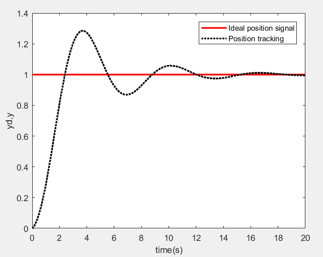
上面代码中比较难懂的可能是计算y的这部分代码，[tCurrent,xCurrent]=ode45(@(t,x) ADRC1_1_4Plant(t,x,para),timeSpan,xInit);%get(t,y)是利用ode45在已经知道初始值xInit和积分区间timeSpan的情况下求出下个时刻的t和x，xInit = xCurrent(length(xCurrent),:);%xInit as the next time begin是把求解出的这些点的最后一个点赋值给xCurrent，来当做下次求值的初始值，y(k)=xInit(1);是把输出y表示出来。然后接下来就是一个误差的比例、积分、微分了。仿真的结果如下：
ode的PID图
（2）欧拉法
欧拉法的原理比较简单，精度也有限，具体想了解的可以看一下知乎上的解答什么是欧拉方法。
还是以上面的系统为例，其离散形式可以写成
$x_1{(k+1)}=x_1{(k)}+hx_2{(k)} & \ x_2{(k+1)}=x_2{(k)}+h(-x_1{(k)}-x_2{(k)}+u(k)) & \ y=x_1{(k)} end{array} right.$
其中h是一个小的常数，按照这种求y的方式，可以直接写出被控对象的PID代码：

复制代码

1
2
3
4
5
6
7
8
9
10
11
12
13
14
15
16
17
18
19
20
21
22
23
24
25
26
27
28
29
30
31
32
33
34
35
36
37
38
39
40
41
42
43
44
45
46
47
48
%Discrete PID control for continuous plant
clear all;
close all;
Kp = 0.5;
Ki = 1;
Kd = 0.5;
loop=2000;


h = 0.01; %constant
e_1=0.0; %last time error
errorSum = 0.0; %the error integral


for k=1:1:loop
    time(k) = k*h;
    inputRef(k)=1; %step signal
    x1(1)=0;
    x2(1)=0;
    u(1)=0;
    
    x1(k+1) = x1(k)+h*x2(k);
    x2(k+1) = x2(k)+h*(-x1(k)-x2(k)+u(k));
    y(k) = x1(k);
       
    e(k)=inputRef(k)-y(k);
    errorSum = errorSum+e(k)*h;
    de(k)=(e(k)-e_1)/h;
    u(k+1)=Kp*e(k) + Ki*errorSum + Kd*de(k);
    %%Control limit
    if u(k)>10.0
        u(k)=10.0;
    end
    if u(k)<-10.0
        u(k)=-10.0;
    end
    
    e_1 = e(k);
end

figure(1);
plot(time,inputRef,'r',time,y,'k:','linewidth',2);
xlabel('time(s)');ylabel('yd,y');
legend('Ideal position signal','Position tracking');
figure(2);
plot(time,inputRef-y,'r','linewidth',2);
xlabel('time(s)'),ylabel('error');

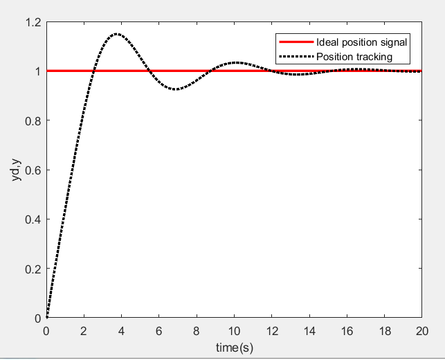
得到的仿真图像与上面的一样，见下图：
PID的欧拉实现
（3）由Z域解得差分方程
这个方法是从先进PID控制与matlab仿真这本书里看到的，具体的做法是先把微分方程写成s域的形式，再转换到z域，利用z反变换写出y的递推公式。
还是以上面的微分方程为例，s域的形式为 $G(s)=frac{1}{s^2+s+1}$ ，再利用matlab的函数c2d变换到z域，利用z域反推递推公式，就能得到y了。代码如下：

复制代码

%the plant transfer function G(s)=1/(s^2+s+1)
clear all;
sampleTime = 0.001; %sample time is 0.001s
sys = tf(1,[1, 1, 1]); %transfer function
discreteSys = c2d(sys, sampleTime,'z'); %from continuous to discrete
[num, den] = tfdata(discreteSys, 'v');
u_1=0.0;
u_2=0.0;
y_1=0.0;
y_2=0.0;
errorSum = 0.0; %the error integral
e_1=0;
Kp=0.5; Ki=1; Kd=0.5;

for k=1:1:20000
    time(k) = k*sampleTime;
    inputRef(k) = 1;
   
    y(k)=-den(2)*y_1-den(3)*y_2+num(2)*u_1+num(3)*u_2;          %实际输出
    
    e(k)=inputRef(k)-y(k);
    errorSum = errorSum+e(k)*sampleTime;
    de(k)=(e(k)-e_1)/sampleTime;
    u(k)=Kp*e(k) + Ki*errorSum + Kd*de(k);
    %%Control limit
    if u(k)>10.0
        u(k)=10.0;
    end
    if u(k)<-10.0
        u(k)=-10.0;
    end
    u_2=u_1;                                                       %保存上上次输入   为下次计算
    u_1=u(k);                                                      %保存上一次控制系数   为下次计算
    y_2=y_1;                                                       %保存上上次输出   为下次计算
    y_1=y(k);                                                   %保存上一次输出   为下次计算
    e_1=e(k);       
end
figure(1);
plot(time,inputRef,'r',time,y,'k:','linewidth',2);
xlabel('time(s)');ylabel('yd,y');
legend('Ideal position signal','Position tracking');
figure(2);
plot(time,inputRef-y,'r','linewidth',2);
xlabel('time(s)'),ylabel('error');

1
2
3
4
5
6
7
8
9
10
11
12
13
14
15
16
17
18
19
20
21
22
23
24
25
26
27
28
29
30
31
32
33
34
35
36
37
38
39
40
41
42
43
44
45
%the plant transfer function G(s)=1/(s^2+s+1)
clear all;
sampleTime = 0.001; %sample time is 0.001s
sys = tf(1,[1, 1, 1]); %transfer function
discreteSys = c2d(sys, sampleTime,'z'); %from continuous to discrete
[num, den] = tfdata(discreteSys, 'v');
u_1=0.0;
u_2=0.0;
y_1=0.0;
y_2=0.0;
errorSum = 0.0; %the error integral
e_1=0;
Kp=0.5; Ki=1; Kd=0.5;

for k=1:1:20000
    time(k) = k*sampleTime;
    inputRef(k) = 1;
   
    y(k)=-den(2)*y_1-den(3)*y_2+num(2)*u_1+num(3)*u_2;          %实际输出
    
    e(k)=inputRef(k)-y(k);
    errorSum = errorSum+e(k)*sampleTime;
    de(k)=(e(k)-e_1)/sampleTime;
    u(k)=Kp*e(k) + Ki*errorSum + Kd*de(k);
    %%Control limit
    if u(k)>10.0
        u(k)=10.0;
    end
    if u(k)<-10.0
        u(k)=-10.0;
    end
    u_2=u_1;                                                       %保存上上次输入   为下次计算
    u_1=u(k);                                                      %保存上一次控制系数   为下次计算
    y_2=y_1;                                                       %保存上上次输出   为下次计算
    y_1=y(k);                                                   %保存上一次输出   为下次计算
    e_1=e(k);       
end
figure(1);
plot(time,inputRef,'r',time,y,'k:','linewidth',2);
xlabel('time(s)');ylabel('yd,y');
legend('Ideal position signal','Position tracking');
figure(2);
plot(time,inputRef-y,'r','linewidth',2);
xlabel('time(s)'),ylabel('error');