序列相加与相乘
-
相加
信号相加的表达式:
x ( n ) = x 1 ( n ) + x 2 ( n ) x(n) = x_1(n) + x_2(n) x(n)=x1(n)+x2(n)clear all; n1 = 0:3; x1 = [2 0.5 0.9 1]; subplot(311); stem(n1,x1); axis([-1 9 0 2.1]); n2 = 0:7; x2 = [0 0.1 0.2 0.3 0.4 0.5 0.6 0.7]; subplot(312); stem(n2,x2) axis([-1 9 0 0.9]); n = 0:7; x1 = [x1 zeros(1,8 - length(n1))]; x2 = [zeros(1,8 - length(n2)) x2]; x = x1 + x2; subplot(313); stem(n,x); axis([-1 9 0 2.1]);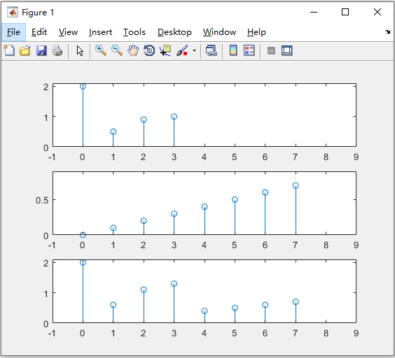
-
相乘
信号相乘的表达式,即两个序列的乘积(或称"点乘"),表达式为:
x ( n ) = x 1 ( n ) ∗ x 2 ( n ) x(n) = x_1(n) * x_2(n) x(n)=x1(n)∗x2(n)clear all; n1 = 0:3; x1 = [3 0.6 0.8 1]; subplot(311); stem(n1,x1); axis([-1 8 0 2.1]); n2 = 0:7; x2 = [0 0.2 0.2 0.3 0.5 0.5 0.6 0.9]; subplot(312); stem(n2,x2); axis([-1 8 0 0.8]); n = 0:7; x1 = [x1 zeros(1,8 - length(n1))]; x2 = [zeros(1,8 - length(n2)) x2]; x = x1 .* x2; subplot(313); stem(n,x); axis([-1 8 0 0.35]);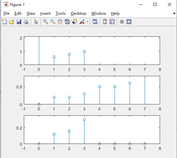
序列累加与序列值乘积
-
序列累加
序列累加式求序列x(n)两点n1和n2之间的所有序列值之和,定义如下:
∑ n = n 1 n 2 x ( n ) = x ( n 1 ) + … … + x ( n 2 ) displaystyle sum^{n_2}_{n=n_1}{x(n)} = x(n_1) + ……+x(n_2) n=n1∑n2x(n)=x(n1)+……+x(n2)n1 = [1 2 3 4]; sum(n1)执行结果:
ans = 10 -
序列乘积
序列值乘积是是x(n)两点n1和n2之间的所有序列值的乘积,定义如下:
∏ n 1 n 2 = x ( n 1 ) ∗ … … ∗ x ( n 2 ) displaystyle prod^{n_2}_{n_1} = x(n_1) * ……* x(n_2) n1∏n2=x(n1)∗……∗x(n2)clear all; x1 = [2 0.5 0.9 2 2]; x = prod(x1)执行结果:
 x =

 	3.6000
序列翻转与序列移位
-
序列翻转
序列翻转表达式: y ( n ) = x ( − n ) y(n)=x(-n) y(n)=x(−n)
 clear all;
 nx = -2:5;
 x = [2 3 4 5 6 7 8 9];
 ny = -fliplr(nx);
 y = fliplr(x);
 subplot(121);
 stem(nx,x,'.');
 axis([-6 6 -1 9]);
 grid on;
 xlabel('n');ylabel('x(n)');
 title('原序列');
 subplot(122);
 stem(ny,y,'.');
 axis([-6 6 -1 9]);
 grid on;
 xlabel('n');ylabel('x(n)');
 title('翻转后的序列');
 set(gcf,'color','w');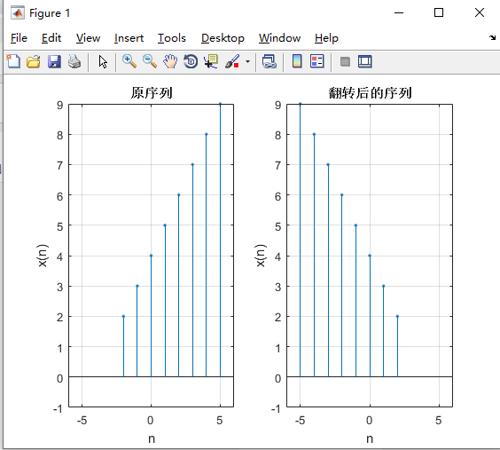
-
序列移位
序列移位表达式: y ( n ) = x ( n − n 0 ) y(n)=x(n-n_0) y(n)=x(n−n0)
 clear all;close all;clc;
 nx = -2:5;
 x = [9 8 7 6 5 5 5 5];
 y = x;
 ny1 = nx + 3;
 ny2 = nx - 2;
 subplot(211);
 stem(nx,x,'.');
 axis([-5 9 -1 6]);
 grid on;
 xlabel('n');
 ylabel('x(n)');
 title('原序列');

 subplot(223);
 stem(ny1,y,'.');
 axis([-5 9 -1 6]);
 grid on;
 xlabel('n');
 ylabel('y1(n)');
 title('右移3位后的序列');

 subplot(224);
 stem(ny2,y,'.');
 axis([-5 9 -1 6]);
 grid on;
 xlabel('n');
 ylabel('y2(n)');
 title('左移2位后的序列');
 set(gcf,'color','w');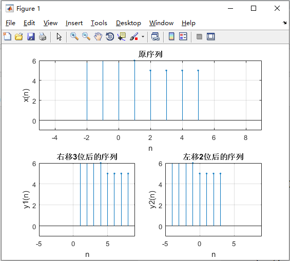
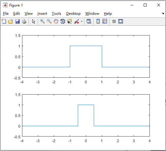
连续时间信号的尺度变换
连续时间信号的尺度变换,是指将信号的横坐标进行扩展或压缩,即将信号f(t)的自变量t更换为at,当a>1时,信号f(at)以原点为基准,沿时间轴压缩到原来的1/a;当a<1时,信号f(at)沿时间轴扩展至原来的1/a倍。
t = -4:0.001:4;
T = 2;
f = rectpuls(t,T);
ft = rectpuls(2*t,T);
subplot(2,1,1);
plot(t,f);
axis([-4 4 -0.5 1.5])
subplot(2,1,2);
plot(t,ft);
axis([-4 4 -0.5 1.5])
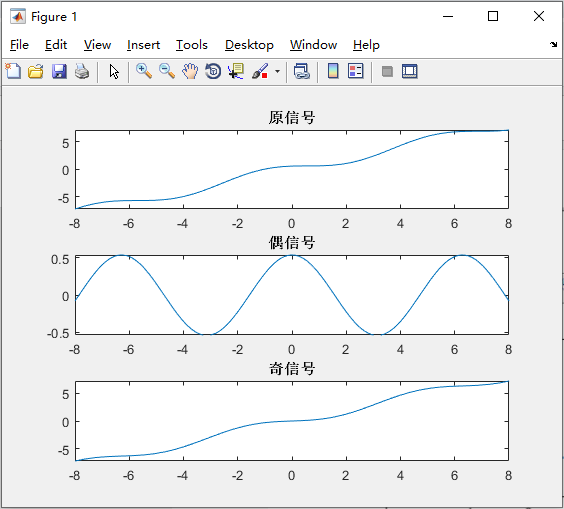
连续时间信号的奇偶分解
信号的奇偶分解原理:任何信号都可以分解为一个偶分量和一个奇分量之和的形式,因为任何信号总可以写成下式:
f
(
t
)
=
1
/
2
[
f
(
t
)
+
f
(
t
)
+
f
(
−
t
)
−
f
(
−
t
)
]
=
1
/
2
[
f
(
t
)
+
f
(
−
t
)
]
+
1
/
2
[
f
(
t
)
−
f
(
−
t
)
]
f(t)=1/2[f(t)+f(t)+f(-t)-f(-t)]=1/2[f(t)+f(-t)]+1/2[f(t)-f(-t)]
f(t)=1/2[f(t)+f(t)+f(−t)−f(−t)]=1/2[f(t)+f(−t)]+1/2[f(t)−f(−t)]
偶分量:
f
e
(
t
)
=
1
/
2
[
f
(
t
)
+
f
(
−
t
)
]
f_e(t)=1/2[f(t)+f(-t)]
fe(t)=1/2[f(t)+f(−t)]
奇分量:
f
o
(
t
)
=
1
/
2
[
f
(
t
)
−
f
(
−
t
)
]
f_o(t)=1/2[f(t)-f(-t)]
fo(t)=1/2[f(t)−f(−t)]
syms t;
f = sym('cos(t + 1) + t');
f1 = subs(f,t,-t);
g = 1/2 * (f + f1);
h = 1/2 * (f - f1);
subplot(311);fplot(f,[-8,8]);title('原信号');
subplot(312);fplot(g,[-8,8]);title('偶信号');
subplot(313);fplot(h,[-8,8]);title('奇信号');
信号的微分和积分
-
微分:对于连续时间信号,其微分运算用函数diff来完成,语法格式:
diff(function,'variable',n)function表示的是要进行求导运算的信号,或者被赋值的符号表达式,variable为求导运算的变量,n为求导的阶数,默认值为一阶导数
 syms t f2;
 f2 = t * (2 * heaviside(t) - heaviside(t - 1)) + heaviside(t - 1);
 t = -1:0.01:2;
 subplot(121);
 ezplot(f2,t);
 title('原函数');
 grid on;
 ylabel('x(t)');
 f = diff(f2,'t',1);
 subplot(122);
 ezplot(f,t);
 title('微分函数');
 grid on;
 ylabel('x(t)');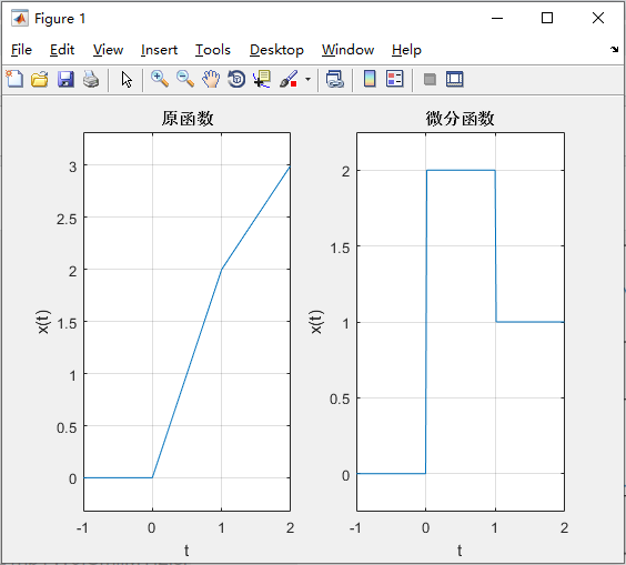
-
积分
连续信号的积分匀速那用函数int来完成,语句格式为int(function,'variable',a,b)其中function表示要进行积分的信号,或者被赋值的符号表达式,variable为求导运算的独立变量,a,b为积分上、下限,a和b被省略时为求不定积分
 syms t f1;
 f1 = 2 * heaviside(t) - heaviside(t - 1);
 t = -1:0.01:2;
 subplot(121);
 ezplot(f1,t);
 title('原函数');
 grid on;
 f = int(f1,'t');
 subplot(122);
 ezplot(f,t);
 grid on;
 title('积分函数');
 ylabel('x(t)');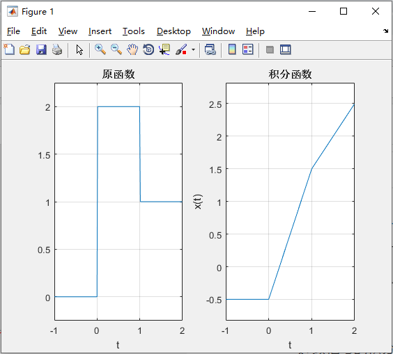
参考文献:
- 《精通MATLAB信号处理》,沈再阳编写,清华大学出版社
最后
以上就是诚心灯泡最近收集整理的关于MATLAB信号处理---学习小案例(4)---信号的基本运算的全部内容,更多相关MATLAB信号处理---学习小案例(4)---信号内容请搜索靠谱客的其他文章。


发表评论 取消回复