- 一、实现卷积 池化 激活 代码
- 1、numpy版本
- 图像生成
- 卷积核生成
- 卷积操作
- 池化操作
- 最大池化
- 平均池化
- 池化在CNN中的作用:
- 最大池化核平均池化效果比较:
- 激活操作:
- 2、pytorch版本(利用pytorch框架)
- 2.1用到的函数
- 2.2代码实现
- 2.1生成图像并定义卷积核
- 2.2 进行卷积操作
- 2.3 进行池化
- 最大池化
- 平均池化
- 2.4 激活函数进行激活
- 3、图像结果可视化
- 二、基于CNN的XO识别
- 1、数据集准备
- 2、 构建模型
- 3、训练模型
- 4、测试训练好的模型
- 5、计算模型的准确率
- 6、查看训练好的模型特征图
- 7、查看训练好的卷积核
- 8、训练模型源代码
- 9、测试源代码
- 9、修改网络模型:
- 思考:为什么模型变小了,反而运算时间增加了?
- 总结:
- 遇到的错误:
一、实现卷积 池化 激活 代码
1、numpy版本
图像生成
生成如下
9
×
9
9times 9
9×9的X型图像:

import numpy as np
#生成图像
def create_pic():
    pic = np.array([[-1, -1, -1, -1, -1, -1, -1, -1, -1],
              [-1, 1, -1, -1, -1, -1, -1, 1, -1],
              [-1, -1, 1, -1, -1, -1, 1, -1, -1],
              [-1, -1, -1, 1, -1, 1, -1, -1, -1],
              [-1, -1, -1, -1, 1, -1, -1, -1, -1],
              [-1, -1, -1, 1, -1, 1, -1, -1, -1],
              [-1, -1, 1, -1, -1, -1, 1, -1, -1],
              [-1, 1, -1, -1, -1, -1, -1, 1, -1],
              [-1, -1, -1, -1, -1, -1, -1, -1, -1]])
    return  pic
卷积核生成
生成课上需要的如下三种卷积核:
#生成三个卷积核
def create_kernel():
    kernel1 = np.array([[1, -1, -1],
                      [-1, 1, -1],
                      [-1, -1, 1]])
    kernel2 = np.array([[1, -1, 1],
                      [-1, 1, -1],
                      [1, -1, 1]])
    kernel3 = np.array([[-1, -1, 1],
                      [-1, 1, -1],
                      [1, -1, -1]])
    Kernel = [kernel1,kernel2,kernel3]
    return Kernel
卷积操作
卷积是对输入信号经过持续的转换, 持续输出另一组信号的过程.,通过卷积生成新函数。输入是固定的蓝色方框和红色框,红色框滑动作为滑动窗口,输出的黑线,代表的是滑动窗口与蓝色框的重叠面积。
代码思路:
生成指定大小的图像,卷积时首先找到图像的对应位置然后进行点乘操作,将卷积后的结果存入到图像中。
'''
参数:传入步长,特征图的大小,原图像,和卷积核
实现操作:初始化特征图==>计算对应卷积的部分的起点和终点==>矩阵对应位置相乘
'''
def conv2d(stride,pic_h,pic_w,picture,Kernel):
feature_map = [0 for i in range(0, 3)] # 初始化3个特征图
for i in range(0, 3):
feature_map[i] = np.zeros((pic_h, pic_w)) # 给特征图进行赋值
for h in range(pic_h): # 向下滑动,得到卷积后的固定行
for w in range(pic_w): # 向右滑动,得到卷积后的固定行的列
h_start = h * stride # 滑动窗口的起始行(高)
h_end = h_start + 3 # 滑动窗口的结束行(高)
h_start = w * stride # 滑动窗口的起始列(宽)
h_end = h_start + 3 # 滑动窗口的结束列(宽)
window = picture[h_start:h_end, h_start:h_end] # 从图切出一个滑动窗口
for i in range(0, 3):
feature_map[i][h, w] = np.divide(np.sum(np.multiply(window, Kernel[i][:, :])), 9)
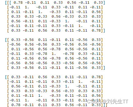
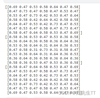
print('=======卷积完毕=======')
print('卷积结果如下:n')
print("特征矩阵:n", np.around(feature_map, decimals=2))
拓展:
填充0,用np.pad()
pad(array, pad_width, mode, **kwargs)
参数解释:
array——表示需要填充的数组;
pad_width——表示每个轴(axis)边缘需要填充的数值数目。
参数输入方式为:((before_1, after_1), … (before_N, after_N)),其中(before_1, after_1)表示第1轴两边缘分别填充before_1个和after_1个数值。取值为:{sequence, array_like, int}
mode——表示填充的方式(取值:str字符串或用户提供的函数),总共有11种填充模式;
mode填充方式:
‘constant’——表示连续填充相同的值,每个轴可以分别指定填充值,constant_values=(x, y)时前面用x填充,后面用y填充,缺省值填充0
‘edge’——表示用边缘值填充
‘linear_ramp’——表示用边缘递减的方式填充
‘maximum’——表示最大值填充
‘mean’——表示均值填充
‘median’——表示中位数填充
‘minimum’——表示最小值填充
‘reflect’——表示对称填充
‘symmetric’——表示对称填充
‘wrap’——表示用原数组后面的值填充前面,前面的值填充后面
在卷积神经网络中,通常采用constant方式进行填充! ! ! ! ! !
池化操作
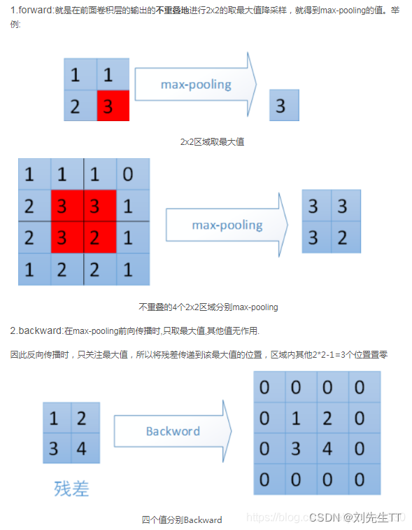
最大池化
前向传播:选图像区域的最大值作为该区域池化后的值。
反向传播:梯度通过最大值的位置传播,其它位置梯度为0
#池化层
def max_pool(picture,stride,h,w):
feature_map_pad_0 = [[0 for i in range(0, 8)] for j in range(0, 8)]
for i in range(0, 3): # 特征图 补 0 ,行 列 都要加 1 (因为上一层是奇数,池化窗口用的偶数)
feature_map_pad_0[i] = np.pad(picture[i], ((0, 1), (0, 1)), 'constant', constant_values=(0, 0))
pooling = [0 for i in range(0, 3)]
for i in range(0, 3):
pooling[i] = np.zeros((h,w)) # 初始化特征图
for h in range(h): # 向下滑动,得到卷积后的固定行
for w in range(w): # 向右滑动,得到卷积后的固定行的列
v_start = h * stride # 滑动窗口的起始行(高)
v_end = v_start + 2 # 滑动窗口的结束行(高)
h_start = w * stride # 滑动窗口的起始列(宽)
h_end = h_start + 2 # 滑动窗口的结束列(宽)
for i in range(0, 3):
pooling[i][h, w] = np.max(feature_map_pad_0[i][v_start:v_end, h_start:h_end])
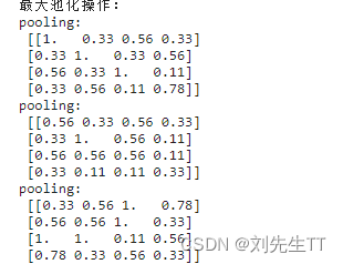
print("======最大池化操作完毕========")
print("pooling:n", np.around(pooling[0], decimals=2))
print("pooling:n", np.around(pooling[1], decimals=2))
print("pooling:n", np.around(pooling[2], decimals=2))
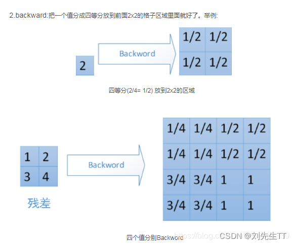
平均池化
前向传播:计算图像区域的平均值作为该区域池化后的值。
反向传播:梯度取均值后分给每个位置。
def aver_pool(picture,stride,h,w):
feature_map_pad_0 = [[0 for i in range(0, 8)] for j in range(0, 8)]
for i in range(0, 3): # 特征图 补 0 ,行 列 都要加 1 (因为上一层是奇数,池化窗口用的偶数)
feature_map_pad_0[i] = np.pad(picture[i], ((0, 1), (0, 1)), 'constant', constant_values=(0, 0))
pooling = [0 for i in range(0, 3)]
for i in range(0, 3):
pooling[i] = np.zeros((h,w)) # 初始化特征图
for h in range(h): # 向下滑动,得到卷积后的固定行
for w in range(w): # 向右滑动,得到卷积后的固定行的列
v_start = h * stride # 滑动窗口的起始行(高)
v_end = v_start + 2 # 滑动窗口的结束行(高)
h_start = w * stride # 滑动窗口的起始列(宽)
h_end = h_start + 2 # 滑动窗口的结束列(宽)
for i in range(0, 3):
pooling[i][h, w] = np.average(feature_map_pad_0[i][v_start:v_end, h_start:h_end])
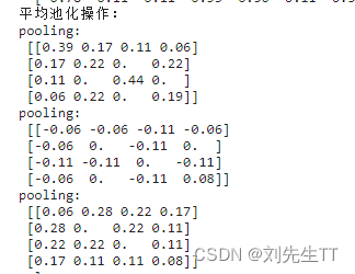
print("======平均池化操作完毕========")
print("pooling:n", np.around(pooling[0], decimals=2))
print("pooling:n", np.around(pooling[1], decimals=2))
print("pooling:n", np.around(pooling[2], decimals=2))
池化在CNN中的作用:
减少维度并可以保留主要特征,类似于PCA,只不过是降维方法有一些差异。
其中最常用的目的是–防止过拟合。提高模型的泛化能力。
最大池化核平均池化效果比较:
通常来讲,最大池化的效果更好,虽然最大池化和平均池化都对数据做了降采样,但是最大池化感觉更像是做了特征选择,选出了分类辨识度更好的特征,提供了非线性,根据相关理论,特征提取的误差主要来自两个方面:(1)邻域大小受限造成的估计值方差增大;(2)卷积层参数误差造成估计均值的偏移。一般来说,平均池化能减小第一种误差,更多的保留图像的背景信息,最大池化能减小第二种误差,更多的保留纹理信息。平均池化更强调对整体特征信息进行一层下采样,在减少参数维度的贡献上更大一点,更多的体现在信息的完整传递这个维度上,一个有代表性的模型,DenseNet中的模块之间的连接大多采用平均池化,在减少维度的同时,更有利信息传递到下一个模块进行特征提取。但是平均池化在全局平均池化操作中应用也比较广,在ResNet和Inception结构中最后一层都使用了平均池化。有的时候在模型接近分类器的末端使用全局平均池化还可以代替Flatten操作,使输入数据变成一位向量。
激活操作:
def relu(x):
return (abs(x) + x) / 2
relu_map_h = 7 # 特征图的高
relu_map_w = 7 # 特征图的宽
relu_map = [0 for i in range(0, 3)] # 初始化3个特征图
for i in range(0, 3):
relu_map[i] = np.zeros((relu_map_h, relu_map_w)) # 初始化特征图
for i in range(0, 3):
relu_map[i] = relu(feature_map[i])
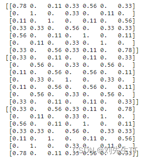
print(np.around(relu_map[0], decimals=2))
print(np.around(relu_map[1], decimals=2))
print(np.around(relu_map[2], decimals=2))
sigmoid激活函数结果
relu激活函数结果
2、pytorch版本(利用pytorch框架)
2.1用到的函数
torch.nn.conv2d(官网链接)
torch.nn.Conv2d(in_channels, out_channels, kernel_size, stride=1, padding=0, dilation=1, groups=1, bias=True)
| 参数 | 参数类型 | ||
|---|---|---|---|
in_channels | int | Number of channels in the input image | 输入图像通道数 |
out_channels | int | Number of channels produced by the convolution | 卷积产生的通道数 |
kernel_size | (int or tuple) | Size of the convolving kernel | 卷积核尺寸,可以设为1个int型数或者一个(int, int)型的元组。例如(2,3)是高2宽3卷积核 |
stride | (int or tuple, optional) | Stride of the convolution. Default: 1 | 卷积步长,默认为1。可以设为1个int型数或者一个(int, int)型的元组。 |
padding | (int or tuple, optional) | Zero-padding added to both sides of the input. Default: 0 | 填充操作,控制padding_mode的数目。 |
padding_mode | (string, optional) | ‘zeros’, ‘reflect’, ‘replicate’ or ‘circular’. Default: ‘zeros’ | padding模式,默认为Zero-padding 。 |
dilation | (int or tuple, optional) | Spacing between kernel elements. Default: 1 | 扩张操作:控制kernel点(卷积核点)的间距,默认值:1。 |
groups | (int, optional) | Number of blocked connections from input channels to output channels. Default: 1 | group参数的作用是控制分组卷积,默认不分组,为1组。 |
bias | (bool, optional) | If True, adds a learnable bias to the output. Default: True | 为真,则在输出中添加一个可学习的偏差。默认:True。 |
torch.nn.MaxPool2d(官网链接)
torch.nn.MaxPool2d(kernel_size,stride,padding,dilation,return_indices,ceil_mode)
| 参数 | 参数类型 | ||
|---|---|---|---|
kernel_size | tuple | 表示做最大池化的窗口大小,可以是单个值,也可以是tuple元组 | |
stride | int | 步长,可以是单个值,也可以是tuple元组 | |
padding | inttuple | 填充,可以是单个值,也可以是tuple元组 | |
dilation | int | 控制窗口中元素步幅 | |
return_indices | bool | 布尔类型,返回最大值位置索引 | |
ceil_mode | bool | 布尔类型,为True,用向上取整的方法,计算输出形状;默认是向下取整。 |
torch.nn.ZeroPad2d(官网链接)
torch.nn.Conv2d(in_channels, out_channels, kernel_size, stride=1, padding=0, dilation=1, groups=1, bias=True)
| 参数 | 参数类型 | |
|---|---|---|
padding | inttuple | 如果是Int,表示四个方向填充多少0.如果是tuple,依此表示左右上下分别田中多少0 |
2.2代码实现
2.1生成图像并定义卷积核
#生成图像,需要四维的图像,符合卷积运算函数
def create_pic():
    picture = torch.tensor([[[[-1, -1, -1, -1, -1, -1, -1, -1, -1],
                    [-1, 1, -1, -1, -1, -1, -1, 1, -1],
                    [-1, -1, 1, -1, -1, -1, 1, -1, -1],
                    [-1, -1, -1, 1, -1, 1, -1, -1, -1],
                    [-1, -1, -1, -1, 1, -1, -1, -1, -1],
                    [-1, -1, -1, 1, -1, 1, -1, -1, -1],
                    [-1, -1, 1, -1, -1, -1, 1, -1, -1],
                    [-1, 1, -1, -1, -1, -1, -1, 1, -1],
                    [-1, -1, -1, -1, -1, -1, -1, -1, -1]]]], dtype=torch.float)
    return picture
def create_kernel():
    conv1 = torch.nn.Conv2d(1, 1, (3, 3), 1)  # in_channel , out_channel , kennel_size , stride
    conv1.weight.data = torch.Tensor([[[[1, -1, -1],
                                        [-1, 1, -1],
                                        [-1, -1, 1]]
                                       ]])
    conv2 = torch.nn.Conv2d(1, 1, (3, 3), 1)  # in_channel , out_channel , kennel_size , stride
    conv2.weight.data = torch.Tensor([[[[1, -1, 1],
                                        [-1, 1, -1],
                                        [1, -1, 1]]
                                       ]])
    conv3 = torch.nn.Conv2d(1, 1, (3, 3), 1)  # in_channel , out_channel , kennel_size , stride
    conv3.weight.data = torch.Tensor([[[[-1, -1, 1],
                                        [-1, 1, -1],
                                        [1, -1, -1]]
                                       ]])
     return conv1,conv2,conv3
2.2 进行卷积操作
feature1 = conv1(picture)
feature2 = conv2(picture)
feature3 = conv3(picture)
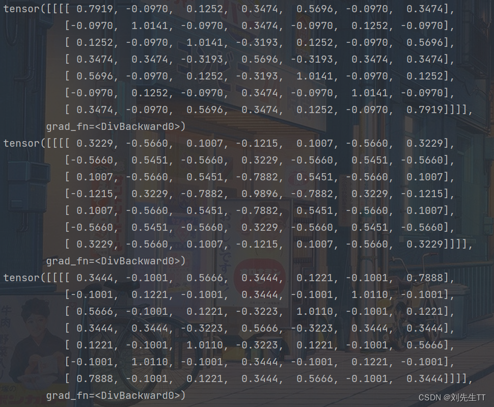
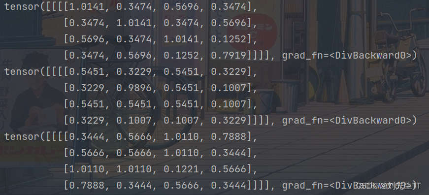
print(feature1 / 9)
print(feature2 / 9)
print(feature3 / 9)
这里为什么除9呢,给大家在这里留一个疑问???
2.3 进行池化
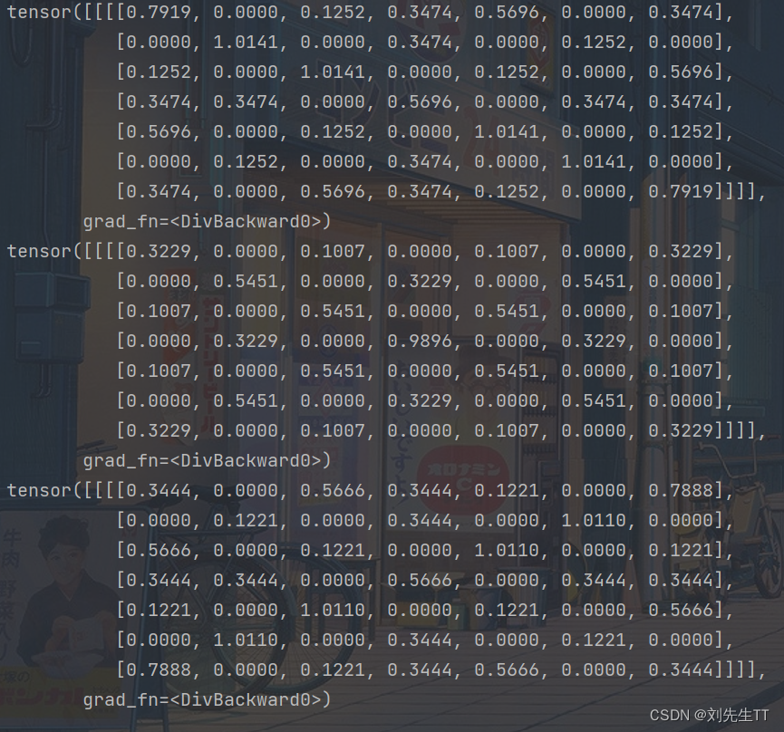
最大池化
max_pool = torch.nn.MaxPool2d(2, padding=0, stride=2)  # Pooling
zeroPad = torch.nn.ZeroPad2d(padding=(0, 1, 0, 1))  # pad 0 , Left Right Up Down
feature_map_pad_0_1 = zeroPad(feature_map1)
feature_pool_1 = max_pool(feature_map_pad_0_1)
feature_map_pad_0_2 = zeroPad(feature_map2)
feature_pool_2 = max_pool(feature_map_pad_0_2)
feature_map_pad_0_3 = zeroPad(feature_map3)
feature_pool_3 = max_pool(feature_map_pad_0_3)
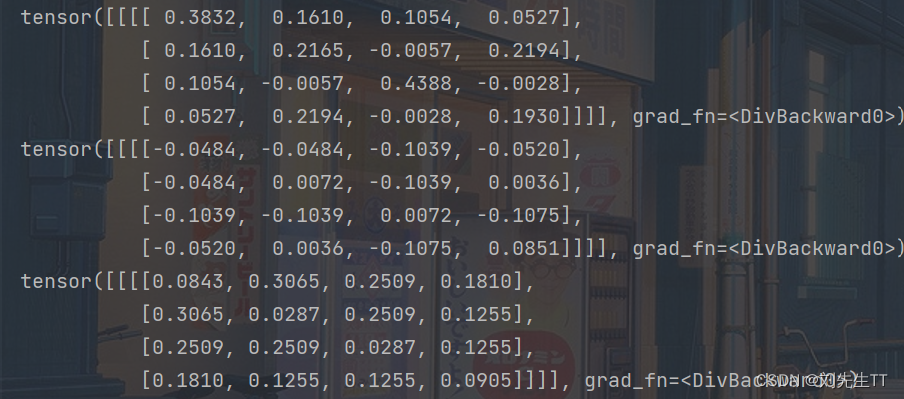
平均池化
avg_pool = torch.nn.AvgPool2d(2, padding=0, stride=2)  # Pooling
zeroPad = torch.nn.ZeroPad2d(padding=(0, 1, 0, 1))  # pad 0 , Left Right Up Down
feature_map_pad_0_1 = zeroPad(feature_map1)
feature_pool_1 = avg_pool(feature_map_pad_0_1)
feature_map_pad_0_2 = zeroPad(feature_map2)
feature_pool_2 = avg_pool(feature_map_pad_0_2)
feature_map_pad_0_3 = zeroPad(feature_map3)
feature_pool_3 = avg_pool(feature_map_pad_0_3)
2.4 激活函数进行激活
activation_function = torch.nn.ReLU()
feature_relu1 = activation_function(feature_map1)
feature_relu2 = activation_function(feature_map2)
feature_relu3 = activation_function(feature_map3)
print(feature_relu1 / 9)
print(feature_relu2 / 9)
print(feature_relu3 / 9)
3、图像结果可视化
可视化这里我们直接调用老师所给的代码。
import torch
import torch.nn as nn
import matplotlib.pyplot as plt
plt.rcParams['font.sans-serif']=['SimHei'] #用来正常显示中文标签
plt.rcParams['axes.unicode_minus']=False #用来正常显示负号 #有中文出现的情况,需要u'内容
x = torch.tensor([[[[-1, -1, -1, -1, -1, -1, -1, -1, -1],
[-1, 1, -1, -1, -1, -1, -1, 1, -1],
[-1, -1, 1, -1, -1, -1, 1, -1, -1],
[-1, -1, -1, 1, -1, 1, -1, -1, -1],
[-1, -1, -1, -1, 1, -1, -1, -1, -1],
[-1, -1, -1, 1, -1, 1, -1, -1, -1],
[-1, -1, 1, -1, -1, -1, 1, -1, -1],
[-1, 1, -1, -1, -1, -1, -1, 1, -1],
[-1, -1, -1, -1, -1, -1, -1, -1, -1]]]], dtype=torch.float)
print(x.shape)
print(x)
img = x.data.squeeze().numpy() # 将输出转换为图片的格式
plt.imshow(img, cmap='gray')
plt.title('原图')
plt.show()
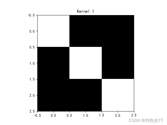
conv1 = nn.Conv2d(1, 1, (3, 3), 1) # in_channel , out_channel , kennel_size , stride
conv1.weight.data = torch.Tensor([[[[1, -1, -1],
[-1, 1, -1],
[-1, -1, 1]]
]])
img = conv1.weight.data.squeeze().numpy() # 将输出转换为图片的格式
plt.imshow(img, cmap='gray')
plt.title('Kernel 1')
plt.show()
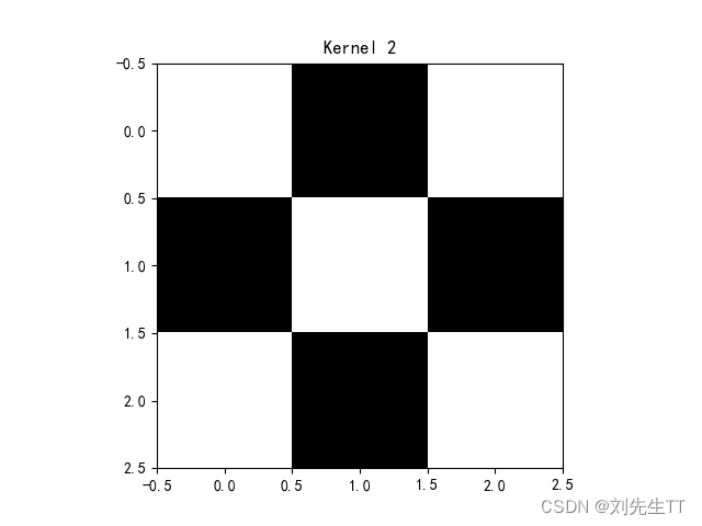
conv2 = nn.Conv2d(1, 1, (3, 3), 1) # in_channel , out_channel , kennel_size , stride
conv2.weight.data = torch.Tensor([[[[1, -1, 1],
[-1, 1, -1],
[1, -1, 1]]
]])
img = conv2.weight.data.squeeze().numpy() # 将输出转换为图片的格式
plt.imshow(img, cmap='gray')
plt.title('Kernel 2')
plt.show()
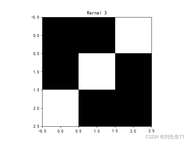
conv3 = nn.Conv2d(1, 1, (3, 3), 1) # in_channel , out_channel , kennel_size , stride
conv3.weight.data = torch.Tensor([[[[-1, -1, 1],
[-1, 1, -1],
[1, -1, -1]]
]])
img = conv3.weight.data.squeeze().numpy() # 将输出转换为图片的格式
plt.imshow(img, cmap='gray')
plt.title('Kernel 3')
plt.show()
feature_map1 = conv1(x)
feature_map2 = conv2(x)
feature_map3 = conv3(x)
print(feature_map1 / 9)
print(feature_map2 / 9)
print(feature_map3 / 9)
img = feature_map1.data.squeeze().numpy() # 将输出转换为图片的格式
plt.imshow(img, cmap='gray')
plt.title('卷积后的特征图1')
plt.show()
print("--------------- 池化 ---------------")
max_pool = nn.MaxPool2d(2, padding=0, stride=2) # Pooling
zeroPad = nn.ZeroPad2d(padding=(0, 1, 0, 1)) # pad 0 , Left Right Up Down
feature_map_pad_0_1 = zeroPad(feature_map1)
feature_pool_1 = max_pool(feature_map_pad_0_1)
feature_map_pad_0_2 = zeroPad(feature_map2)
feature_pool_2 = max_pool(feature_map_pad_0_2)
feature_map_pad_0_3 = zeroPad(feature_map3)
feature_pool_3 = max_pool(feature_map_pad_0_3)
print(feature_pool_1.size())
print(feature_pool_1 / 9)
print(feature_pool_2 / 9)
print(feature_pool_3 / 9)
img = feature_pool_1.data.squeeze().numpy() # 将输出转换为图片的格式
plt.imshow(img, cmap='gray')
plt.title('卷积池化后的特征图1')
plt.show()
print("--------------- 激活 ---------------")
activation_function = nn.ReLU()
feature_relu1 = activation_function(feature_map1)
feature_relu2 = activation_function(feature_map2)
feature_relu3 = activation_function(feature_map3)
print(feature_relu1 / 9)
print(feature_relu2 / 9)
print(feature_relu3 / 9)
img = feature_relu1.data.squeeze().numpy() # 将输出转换为图片的格式
plt.imshow(img, cmap='gray')
plt.title('卷积 + relu 后的特征图1')
plt.show()
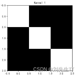
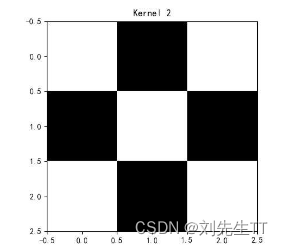
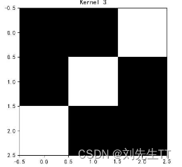
卷积操作如下:
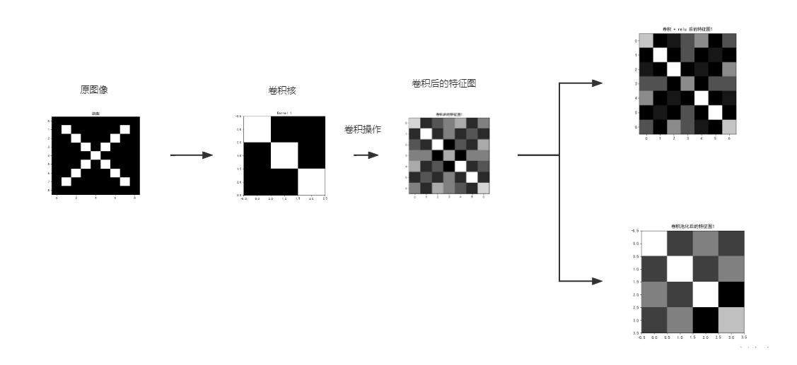
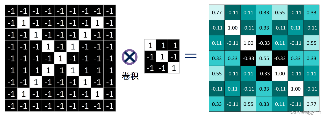
和上课所给结果一致,其中1表示与特征相似度大,-1表示与特征差异度大,0表示与特征无关。下面是三种卷积核的图像可视化。
二、基于CNN的XO识别
1、数据集准备
数据集下载地址:https://download.csdn.net/download/qq_51698536/86799231
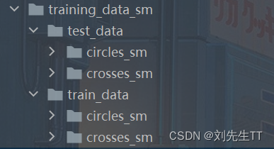
数据集的分级目录:
采用机器学习中数据集的分割方法:抽中其中15%的数据用作测试集,85%的数据用作训练集。
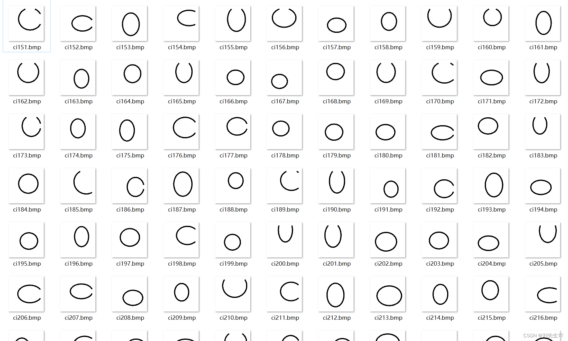
部分数据集展示:
训练集中为O的图像:
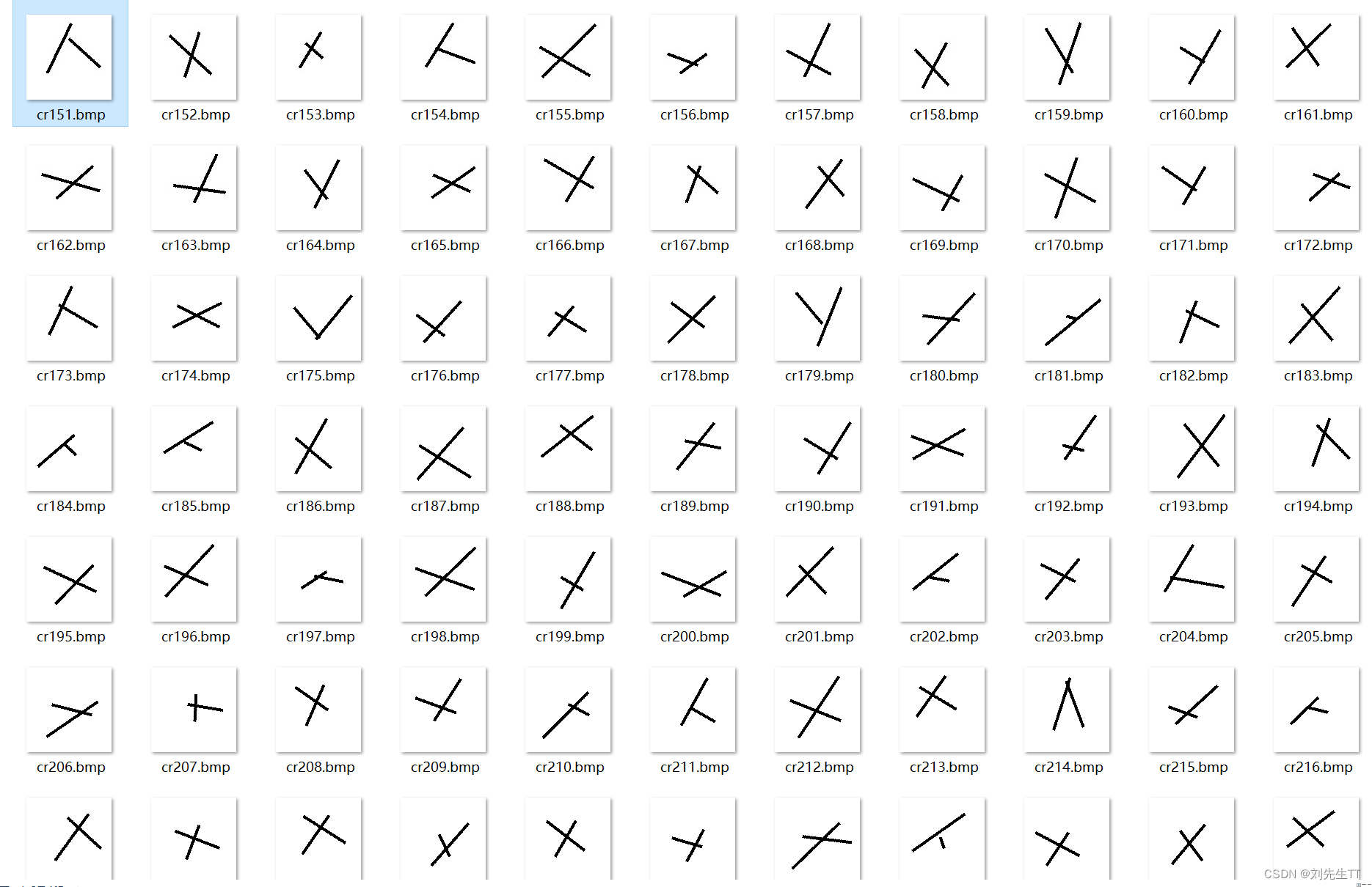
训练集中为X的图像:
2、 构建模型
首先是老师上课所给的模型(可能是最好的,也可能是老师给下的套,最后会自己斟酌更改一下网络):
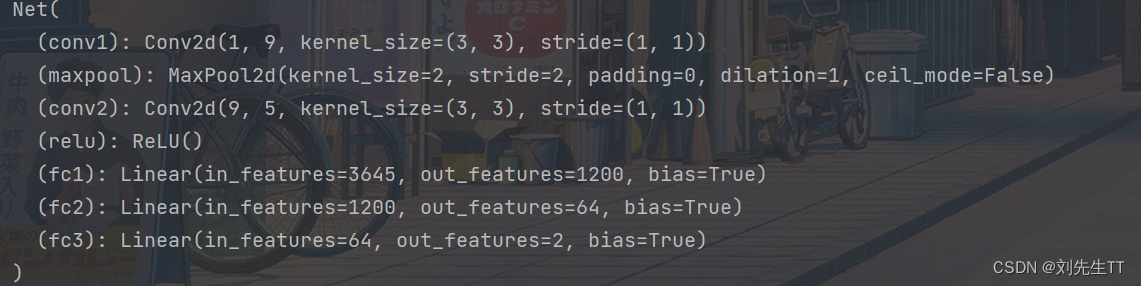
class Net(nn.Module):
    def __init__(self):
        super(Net, self).__init__()
        self.conv1 = nn.Conv2d(1, 9, 3)
        self.maxpool = nn.MaxPool2d(2, 2)
        self.conv2 = nn.Conv2d(9, 5, 3)

        self.relu = nn.ReLU()
        self.fc1 = nn.Linear(27 * 27 * 5, 1200)
        self.fc2 = nn.Linear(1200, 64)
        self.fc3 = nn.Linear(64, 2)

    def forward(self, x):
        x = self.maxpool(self.relu(self.conv1(x)))
        x = self.maxpool(self.relu(self.conv2(x)))
        x = x.view(-1, 27 * 27 * 5)
        x = self.relu(self.fc1(x))
        x = self.relu(self.fc2(x))
        x = self.fc3(x)
        return x
3、训练模型
model = Net()
criterion = torch.nn.CrossEntropyLoss() # 损失函数 交叉熵损失函数
optimizer = optim.SGD(model.parameters(), lr=0.1) # 优化函数:随机梯度下降
epochs = 10
for epoch in range(epochs):
running_loss = 0.0
for i, data in enumerate(data_loader):
images, label = data
out = model(images)
loss = criterion(out, label)
optimizer.zero_grad()
loss.backward()
optimizer.step()
running_loss += loss.item()
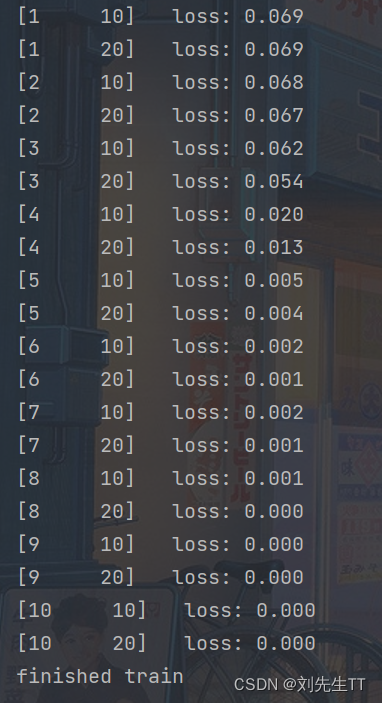
if (i + 1) % 10 == 0:
print('[%d %5d] loss: %.3f' % (epoch + 1, i + 1, running_loss / 100))
running_loss = 0.0
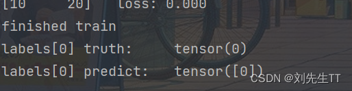
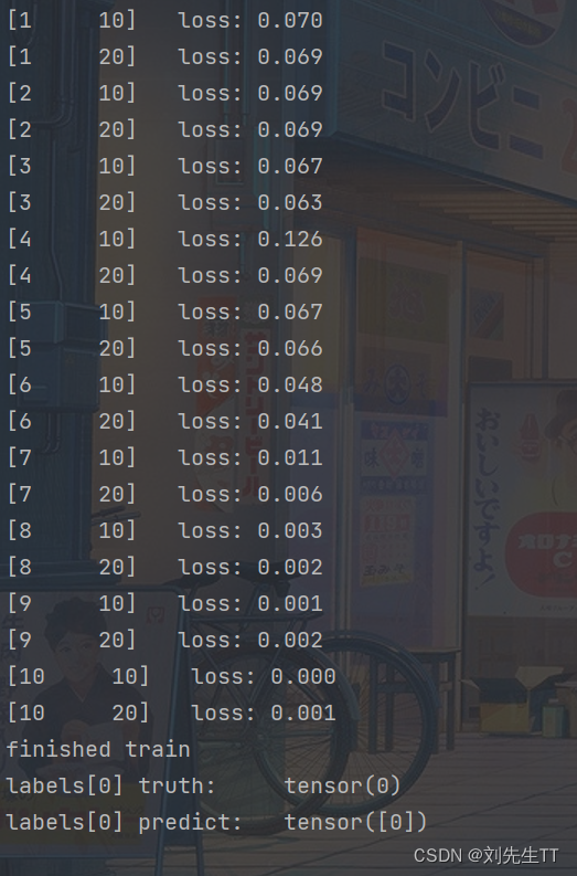
print('finished train')
# 保存模型
torch.save(model, 'model_name.pth') # 保存的是模型, 不止是w和b权重值
4、测试训练好的模型
# 读取模型
model_load = torch.load('model_name.pth')
# 读取一张图片 images[0],测试
print("labels[0] truth:t", labels[0])
x = images[0]
predicted = torch.max(model_load(x), 1)
print("labels[0] predict:t", predicted.indices)
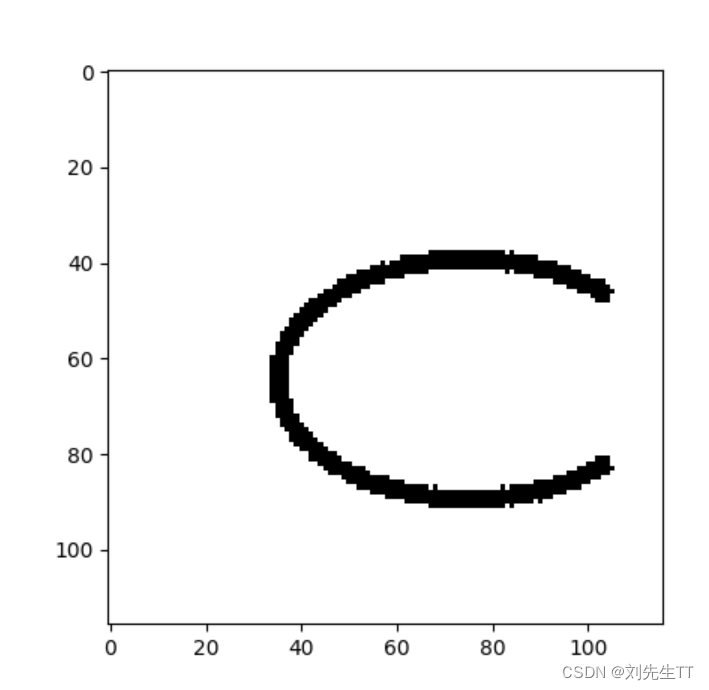
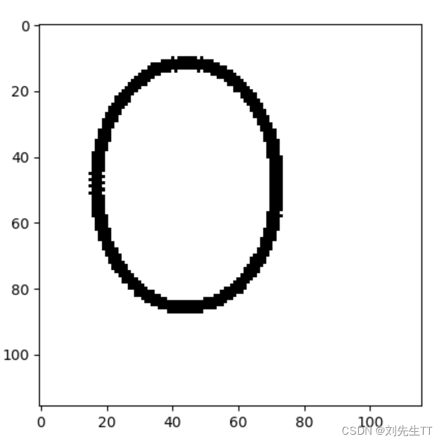
img = images[0].data.squeeze().numpy() # 将输出转换为图片的格式
plt.imshow(img, cmap='gray')
plt.show()
5、计算模型的准确率
# 读取模型
model_load = torch.load('model_name1.pth')

correct = 0
total = 0
with torch.no_grad():  # 进行评测的时候网络不更新梯度
    for data in data_loader_test:  # 读取测试集
        images, labels = data
        outputs = model_load(images)
        _, predicted = torch.max(outputs.data, 1)  # 取出 最大值的索引 作为 分类结果
        total += labels.size(0)  # labels 的长度
        correct += (predicted == labels).sum().item()  # 预测正确的数目
print('Accuracy of the network on the  test images: %f %%' % (100. * correct / total))
6、查看训练好的模型特征图
# 看看每层的 卷积核 长相,特征图 长相
# 获取网络结构的特征矩阵并可视化
import torch
import matplotlib.pyplot as plt
import numpy as np
from PIL import Image
from torchvision import transforms, datasets
import torch.nn as nn
from torch.utils.data import DataLoader

#  定义图像预处理过程(要与网络模型训练过程中的预处理过程一致)

transforms = transforms.Compose([
    transforms.ToTensor(),  # 把图片进行归一化,并把数据转换成Tensor类型
    transforms.Grayscale(1)  # 把图片 转为灰度图
])
path = r'training_data_sm'
data_train = datasets.ImageFolder(path, transform=transforms)
data_loader = DataLoader(data_train, batch_size=64, shuffle=True)
for i, data in enumerate(data_loader):
    images, labels = data
    print(images.shape)
    print(labels.shape)
    break


class Net(nn.Module):
    def __init__(self):
        super(Net, self).__init__()
        self.conv1 = nn.Conv2d(1, 9, 3)  # in_channel , out_channel , kennel_size , stride
        self.maxpool = nn.MaxPool2d(2, 2)
        self.conv2 = nn.Conv2d(9, 5, 3)  # in_channel , out_channel , kennel_size , stride

        self.relu = nn.ReLU()
        self.fc1 = nn.Linear(27 * 27 * 5, 1200)  # full connect 1
        self.fc2 = nn.Linear(1200, 64)  # full connect 2
        self.fc3 = nn.Linear(64, 2)  # full connect 3

    def forward(self, x):
        outputs = []
        x = self.conv1(x)
        outputs.append(x)
        x = self.relu(x)
        outputs.append(x)
        x = self.maxpool(x)
        outputs.append(x)
        x = self.conv2(x)

        x = self.relu(x)

        x = self.maxpool(x)

        x = x.view(-1, 27 * 27 * 5)
        x = self.relu(self.fc1(x))
        x = self.relu(self.fc2(x))
        x = self.fc3(x)
        return outputs


# create model
model1 = Net()

# load model weights加载预训练权重
# model_weight_path ="./AlexNet.pth"
model_weight_path = "model_name1.pth"
model1.load_state_dict(torch.load(model_weight_path))

# 打印出模型的结构
print(model1)

x = images[0]

# forward正向传播过程
out_put = model1(x)

for feature_map in out_put:
    # [N, C, H, W] -> [C, H, W]    维度变换
    im = np.squeeze(feature_map.detach().numpy())
    # [C, H, W] -> [H, W, C]
    im = np.transpose(im, [1, 2, 0])
    print(im.shape)

    # show 9 feature maps
    plt.figure()
    for i in range(9):
        ax = plt.subplot(3, 3, i + 1)  # 参数意义:3:图片绘制行数,5:绘制图片列数,i+1:图的索引
        # [H, W, C]
        # 特征矩阵每一个channel对应的是一个二维的特征矩阵,就像灰度图像一样,channel=1
        # plt.imshow(im[:, :, i])
        plt.imshow(im[:, :, i], cmap='gray')
    plt.show()
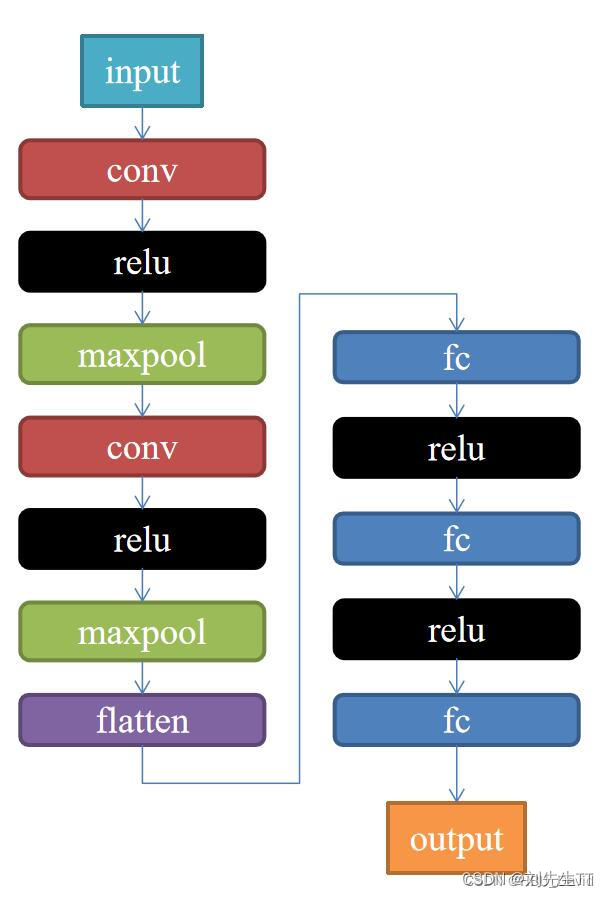
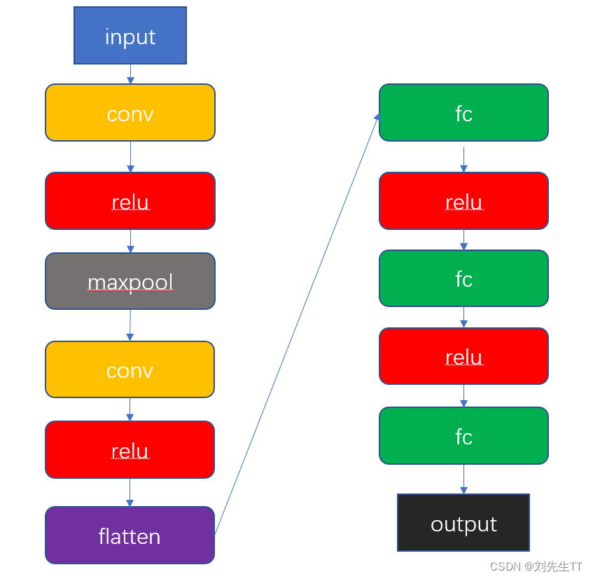
网络模型如下:
第一轮卷积后的特征图
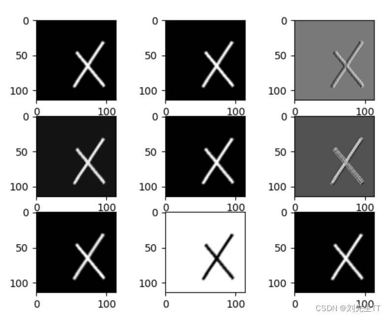
通过特征图我们可以发现,第一轮卷积以后经能提取大部分特征了,不同的卷积核提取的特征结果不同。
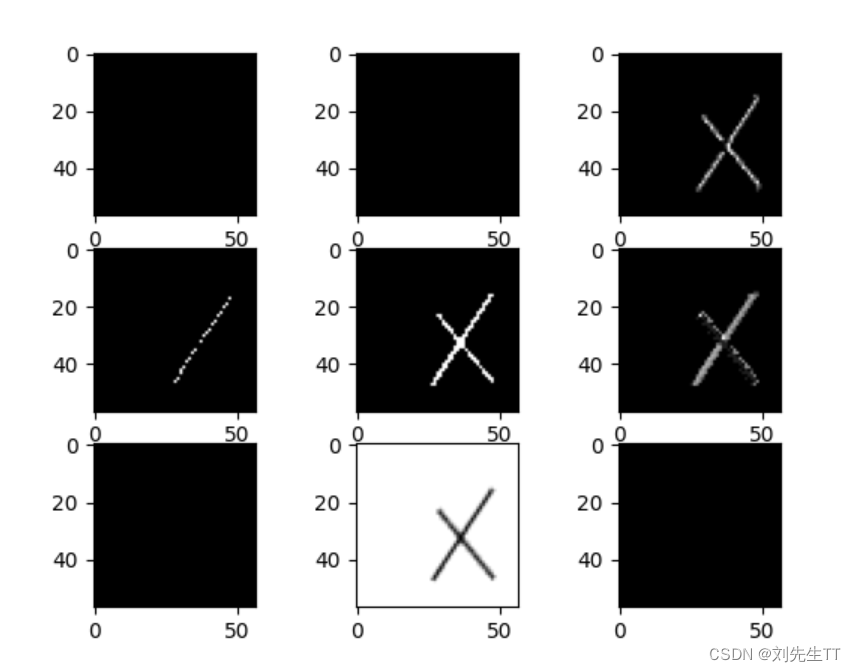
最大池化后图像
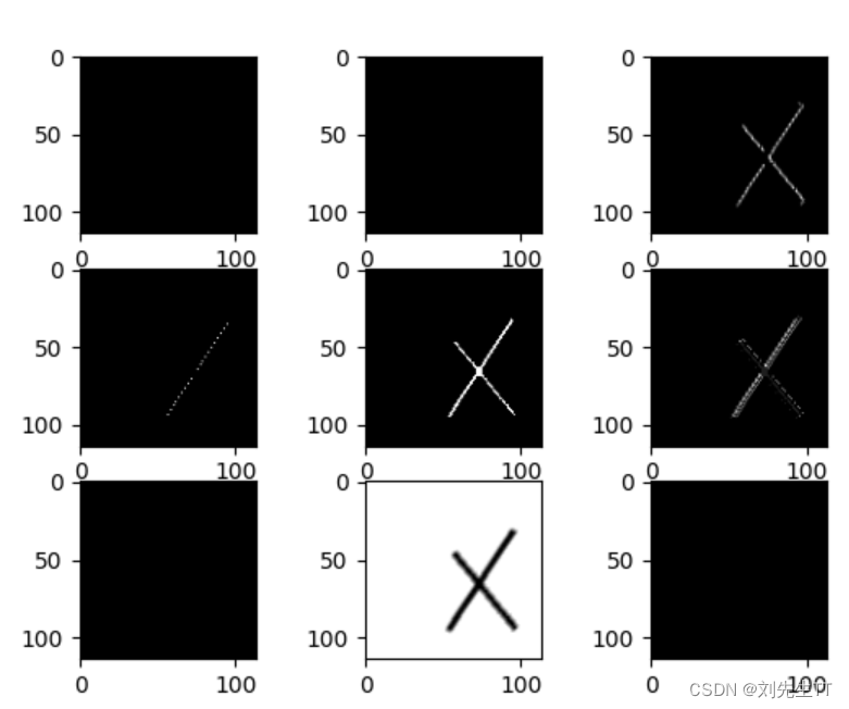
第二轮卷积后的图像
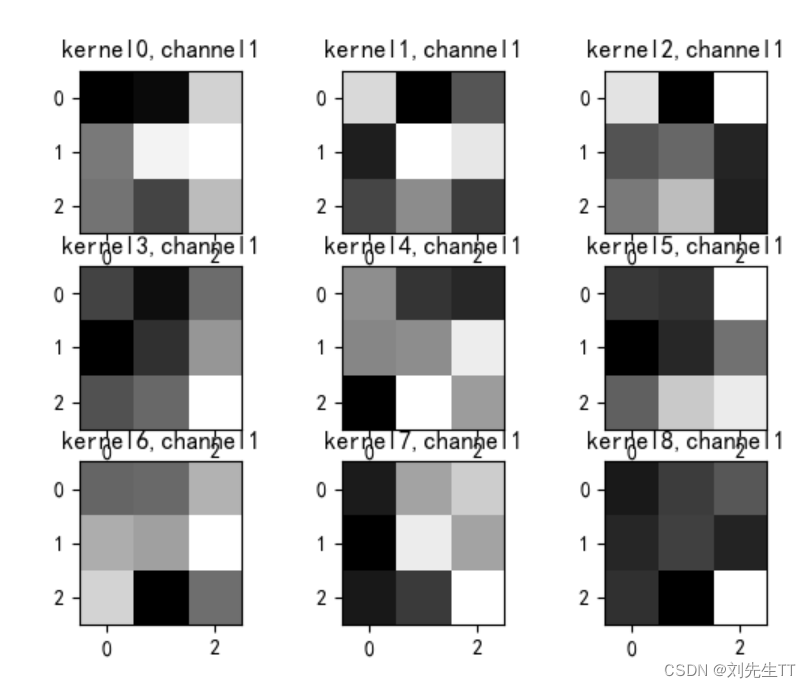
7、查看训练好的卷积核
# 看看每层的 卷积核 长相,特征图 长相
# 获取网络结构的特征矩阵并可视化
import torch
import matplotlib.pyplot as plt
import numpy as np
from PIL import Image
from torchvision import transforms, datasets
import torch.nn as nn
from torch.utils.data import DataLoader

plt.rcParams['font.sans-serif'] = ['SimHei']  # 用来正常显示中文标签
plt.rcParams['axes.unicode_minus'] = False  # 用来正常显示负号 #有中文出现的情况,需要u'内容
#  定义图像预处理过程(要与网络模型训练过程中的预处理过程一致)
transforms = transforms.Compose([
    transforms.ToTensor(),  # 把图片进行归一化,并把数据转换成Tensor类型
    transforms.Grayscale(1)  # 把图片 转为灰度图
])
path = r'train_data'
data_train = datasets.ImageFolder(path, transform=transforms)
data_loader = DataLoader(data_train, batch_size=64, shuffle=True)
for i, data in enumerate(data_loader):
    images, labels = data
    # print(images.shape)
    # print(labels.shape)
    break


class Net(nn.Module):
    def __init__(self):
        super(Net, self).__init__()
        self.conv1 = nn.Conv2d(1, 9, 3)  # in_channel , out_channel , kennel_size , stride
        self.maxpool = nn.MaxPool2d(2, 2)
        self.conv2 = nn.Conv2d(9, 5, 3)  # in_channel , out_channel , kennel_size , stride

        self.relu = nn.ReLU()
        self.fc1 = nn.Linear(27 * 27 * 5, 1200)  # full connect 1
        self.fc2 = nn.Linear(1200, 64)  # full connect 2
        self.fc3 = nn.Linear(64, 2)  # full connect 3

    def forward(self, x):
        outputs = []
        x = self.maxpool(self.relu(self.conv1(x)))
        # outputs.append(x)
        x = self.maxpool(self.relu(self.conv2(x)))
        outputs.append(x)
        x = x.view(-1, 27 * 27 * 5)
        x = self.relu(self.fc1(x))
        x = self.relu(self.fc2(x))
        x = self.fc3(x)
        return outputs


# create model
model1 = Net()

# load model weights加载预训练权重
model_weight_path = "model_name.pth"
model1.load_state_dict(torch.load(model_weight_path))

x = images[0]
x =torch.unsqueeze(x, dim=0)

# forward正向传播过程
out_put = model1(x)

weights_keys = model1.state_dict().keys()
for key in weights_keys:
    print("key :", key)
    # 卷积核通道排列顺序 [kernel_number, kernel_channel, kernel_height, kernel_width]
    if key == "conv1.weight":
        weight_t = model1.state_dict()[key].numpy()
        print("weight_t.shape", weight_t.shape)
        k = weight_t[:, 0, :, :]  # 获取第一个卷积核的信息参数
        # show 9 kernel ,1 channel
        plt.figure()

        for i in range(9):
            ax = plt.subplot(3, 3, i + 1)  # 参数意义:3:图片绘制行数,5:绘制图片列数,i+1:图的索引
            plt.imshow(k[i, :, :], cmap='gray')
            title_name = 'kernel' + str(i) + ',channel1'
            plt.title(title_name)
        plt.show()

    if key == "conv2.weight":
        weight_t = model1.state_dict()[key].numpy()
        print("weight_t.shape", weight_t.shape)
        k = weight_t[:, :, :, :]  # 获取第一个卷积核的信息参数
        print(k.shape)
        print(k)

        plt.figure()
        for c in range(9):
            channel = k[:, c, :, :]
            for i in range(5):
                ax = plt.subplot(2, 3, i + 1)  # 参数意义:3:图片绘制行数,5:绘制图片列数,i+1:图的索引
                plt.imshow(channel[i, :, :], cmap='gray')
                title_name = 'kernel' + str(i) + ',channel' + str(c)
                plt.title(title_name)
            plt.show()
第一轮训练后卷积核
8、训练模型源代码
# https://blog.csdn.net/qq_53345829/article/details/124308515
import torch
from torchvision import transforms, datasets
import torch.nn as nn
from torch.utils.data import DataLoader
import matplotlib.pyplot as plt
import torch.optim as optim
transforms = transforms.Compose([
transforms.ToTensor(), # 把图片进行归一化,并把数据转换成Tensor类型
transforms.Grayscale(1) # 把图片 转为灰度图
])
path = r'train_data'
path_test = r'test_data'
data_train = datasets.ImageFolder(path, transform=transforms)
data_test = datasets.ImageFolder(path_test, transform=transforms)
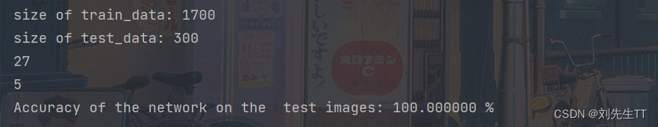
print("size of train_data:", len(data_train))
print("size of test_data:", len(data_test))
data_loader = DataLoader(data_train, batch_size=64, shuffle=True)
data_loader_test = DataLoader(data_test, batch_size=64, shuffle=True)
for i, data in enumerate(data_loader):
images, labels = data
print(images.shape)
print(labels.shape)
break
for i, data in enumerate(data_loader_test):
images, labels = data
print(images.shape)
print(labels.shape)
break
class Net(nn.Module):
def __init__(self):
super(Net, self).__init__()
self.conv1 = nn.Conv2d(1, 9, 3) # in_channel , out_channel , kennel_size , stride
self.maxpool = nn.MaxPool2d(2, 2)
self.conv2 = nn.Conv2d(9, 5, 3) # in_channel , out_channel , kennel_size , stride
self.relu = nn.ReLU()
self.fc1 = nn.Linear(27 * 27 * 5, 1200) # full connect 1
self.fc2 = nn.Linear(1200, 64) # full connect 2
self.fc3 = nn.Linear(64, 2) # full connect 3
def forward(self, x):
x = self.maxpool(self.relu(self.conv1(x)))
x = self.maxpool(self.relu(self.conv2(x)))
x = x.view(-1, 27 * 27 * 5)
x = self.relu(self.fc1(x))
x = self.relu(self.fc2(x))
x = self.fc3(x)
return x
model = Net()
criterion = torch.nn.CrossEntropyLoss() # 损失函数 交叉熵损失函数
optimizer = optim.SGD(model.parameters(), lr=0.1) # 优化函数:随机梯度下降
epochs = 10
for epoch in range(epochs):
running_loss = 0.0
for i, data in enumerate(data_loader):
images, label = data
out = model(images)
loss = criterion(out, label)
optimizer.zero_grad()
loss.backward()
optimizer.step()
running_loss += loss.item()
if (i + 1) % 10 == 0:
print('[%d %5d] loss: %.3f' % (epoch + 1, i + 1, running_loss / 100))
running_loss = 0.0
print('finished train')
# 保存模型 torch.save(model.state_dict(), model_path)
torch.save(model.state_dict(), 'model_name.pth') # 保存的是模型, 不止是w和b权重值
# 读取一张图片 images[0],测试
print("labels[0] truth:t", labels[0])
x = images[0]
x =torch.unsqueeze(x, dim=0)
predicted = torch.max(model(x), 1)
print("labels[0] predict:t", predicted.indices)
img = images[0].data.squeeze().numpy() # 将输出转换为图片的格式
plt.imshow(img, cmap='gray')
plt.show()
9、测试源代码
# https://blog.csdn.net/qq_53345829/article/details/124308515
import torch
from torchvision import transforms, datasets
import torch.nn as nn
from torch.utils.data import DataLoader
import matplotlib.pyplot as plt
import torch.optim as optim

transforms = transforms.Compose([
    transforms.ToTensor(),  # 把图片进行归一化,并把数据转换成Tensor类型
    transforms.Grayscale(1)  # 把图片 转为灰度图
])

path = r'train_data'
path_test = r'test_data'

data_train = datasets.ImageFolder(path, transform=transforms)
data_test = datasets.ImageFolder(path_test, transform=transforms)

print("size of train_data:", len(data_train))
print("size of test_data:", len(data_test))

data_loader = DataLoader(data_train, batch_size=64, shuffle=True)
data_loader_test = DataLoader(data_test, batch_size=64, shuffle=True)
print(len(data_loader))
print(len(data_loader_test))


class Net(nn.Module):
    def __init__(self):
        super(Net, self).__init__()
        self.conv1 = nn.Conv2d(1, 9, 3)  # in_channel , out_channel , kennel_size , stride
        self.maxpool = nn.MaxPool2d(2, 2)
        self.conv2 = nn.Conv2d(9, 5, 3)  # in_channel , out_channel , kennel_size , stride

        self.relu = nn.ReLU()
        self.fc1 = nn.Linear(27 * 27 * 5, 1200)  # full connect 1
        self.fc2 = nn.Linear(1200, 64)  # full connect 2
        self.fc3 = nn.Linear(64, 2)  # full connect 3

    def forward(self, x):
        x = self.maxpool(self.relu(self.conv1(x)))
        x = self.maxpool(self.relu(self.conv2(x)))
        x = x.view(-1, 27 * 27 * 5)
        x = self.relu(self.fc1(x))
        x = self.relu(self.fc2(x))
        x = self.fc3(x)
        return x


# 读取模型
model = Net()
model.load_state_dict(torch.load('model_name.pth', map_location='cpu'))  # 导入网络的参数

# model_load = torch.load('model_name1.pth')
# https://blog.csdn.net/qq_41360787/article/details/104332706

correct = 0
total = 0
with torch.no_grad():  # 进行评测的时候网络不更新梯度
    for data in data_loader_test:  # 读取测试集
        images, labels = data
        outputs = model(images)
        _, predicted = torch.max(outputs.data, 1)  # 取出 最大值的索引 作为 分类结果
        total += labels.size(0)  # labels 的长度
        correct += (predicted == labels).sum().item()  # 预测正确的数目
print('Accuracy of the network on the  test images: %f %%' % (100. * correct / total))

#  "_," 的解释 https://blog.csdn.net/weixin_48249563/article/details/111387501
9、修改网络模型:
网络模型代码修改如下:
class Net(nn.Module):
    def __init__(self):
        super(Net, self).__init__()
        self.conv1 = nn.Conv2d(1, 9, 3)  # in_channel , out_channel , kennel_size , stride
        self.maxpool = nn.MaxPool2d(2, 2)
        self.conv2 = nn.Conv2d(9, 5, 3)  # in_channel , out_channel , kennel_size , stride

        self.relu = nn.ReLU()
        self.fc1 = nn.Linear(55 * 55 * 5, 1200)  # full connect 1
        self.fc2 = nn.Linear(1200, 64)  # full connect 2
        self.fc3 = nn.Linear(64, 2)  # full connect 3

    def forward(self, x):
        x = self.maxpool(self.relu(self.conv1(x)))
        x = self.maxpool(self.relu(self.conv2(x)))
        x = x.view(-1,  55* 55 * 5)
        x = self.relu(self.fc1(x))
        x = self.relu(self.fc2(x))
        x = self.fc3(x)
        return x
训练结果如下:
思考:为什么模型变小了,反而运算时间增加了?
但是这里通过思考,我们可以发现,两种网络虽然准确率差不多,但是训练时间明显多了一半这是为什么呢?


答:我的看法,虽然去掉了最大池化层,但是图片中并没有少了一倍的像素,在后续的计算中仍然花费了大量的时间,如果具有最大池化层,虽然多了一层计算,但是这一层计算能帮助我们减少了一般的像素点,相对来说,减少这一半像素点之后所花费的时间比最大池化层所花费的时间更少,所以老师的模型花费的时间更小一下。看来老师这次并没有下套,所给的模型相对来说还是比较好的。哈哈哈
python时间计算函数:
import datetime
start = datetime.datetime.now()
运行代码
end = datetime.datetime.now()
print('totally time is ',end - start)
总结:
通过本次实验,自己使用Numpy手写底层代码(当然大部分还是参考了老师的代码,百分百自己写的代码咋看咋别扭)和使用框架进行卷积池化操作,还是框架简单一些,但是专业人士又不得不得会底层代码,写底层代码太浪费时间了,在第一部分进行池化操作和卷积操作的时候,发现池化和卷积提取的主要特征是不同,我觉得卷积主要是提取特征,而池化主要偏向于降维,在第二部分的时候,我们又对卷积核进行进一步得了了解,这里是端到端的学习,也就是人们口中的深度学习了,我们发现不同的卷积核提取的主要特征还不同,看来提取特征这里面的学问还很大,再进行更改的模型的时候,也对为什么少了一层池化层,反而运算时间变长了,前提是我电脑应该没有选择性卡顿这一说法哈。
遇到的错误:
1、图像和网络维度不一致,需要将三维图像变成四维:
x =torch.unsqueeze(x, dim=0)
2、手忙脚乱
为什么说手忙脚乱也是一个错误呢,因为在使用Numpy手写底层代码的时候,我想自己一个人完成,不参考老师的代码,同时又懒懒得做流程图,导致半天过去了一直拆东墙补西墙,丢了西瓜捡芝麻。
最后
以上就是失眠睫毛膏最近收集整理的关于NNDL 作业6:基于CNN的XO识别的全部内容,更多相关NNDL内容请搜索靠谱客的其他文章。


发表评论 取消回复