Python机器学习08——决策树算法

本系列所有的代码和数据都可以从陈强老师的个人主页上下载：Python数据程序

参考书目：陈强.机器学习及Python应用. 北京：高等教育出版社, 2021.

本系列基本不讲数学原理，只从代码角度去让读者们利用最简洁的Python代码实现机器学习方法。

本章继续非参数的方法——决策树。决策树方法很早就成熟了，因为它直观便捷，和计算机的一些底层逻辑结构很像，一直都有广泛的应用。其最早有ID3、C4.5、C5.0、CART等等。但其实都大同小异，损失函数不一样而已，还有分裂节点个数不一样。CRAT算法是二叉树，数学本质就是切割样本取值空间。因此决策树的决策边界都是矩形区域，（类似楼梯），下面会一一展示。同样决策树可以用于分类和回归问题。分类问题叫分类树。回归问题叫回归树。决策树还有一个优点在于可以度量变量的重要性。就是可以了解到变量x1,x2,x3,x4.....谁对y的影响最大。这是线性回归给不了的，而且线性回归假设太多，决策树就基本没有，所以适用范围更广。首先介绍回归树。

回归树Python案例

还是导入包和数据，采用回归问题常用的波士顿房价数据集：

import numpy as np
import pandas as pd
import matplotlib.pyplot as plt
import seaborn as sns
from sklearn.model_selection import train_test_split
from sklearn.model_selection import KFold, StratifiedKFold
from sklearn.model_selection import GridSearchCV
from sklearn.tree import DecisionTreeRegressor,export_text
from sklearn.tree import DecisionTreeClassifier, plot_tree
from sklearn.datasets import load_boston
from sklearn.metrics import cohen_kappa_score

Boston=load_boston()
Boston.feature_names
#波士顿房价数据集在sklearn库后面版本可能被移除...因为有种族问题...可以用下面的方法替代

data_url = "http://lib.stat.cmu.edu/datasets/boston"
raw_df = pd.read_csv(data_url, sep="s+", skiprows=22, header=None)
data = np.hstack([raw_df.values[::2, :], raw_df.values[1::2, :2]])
target = raw_df.values[1::2, 2]

数据在线性回归那一节展示过了，现在就直接开始划分训练集和测试集，然后拟合评价，打印出决策树

# Data Preparation
X_train, X_test, y_train, y_test = train_test_split(data,target, test_size=0.3, random_state=0)

# Regression Tree 
model = DecisionTreeRegressor(max_depth=2, random_state=123)
model.fit(X_train, y_train)
model.score(X_test, y_test)

#打印决策树
print(export_text(model,feature_names=list(Boston.feature_names)))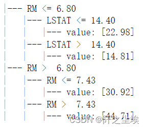

 sklearn还支持直接画决策树的图：

plot_tree(model, feature_names=Boston.feature_names, node_ids=True, rounded=True, precision=2)
plt.tight_layout()
plt.savefig('tree.png',dpi=200)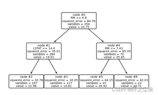

 决策树也是可以进行正则化的，防止过拟合，减低模型复杂度。惩罚系数和决策树的损失可视化：

# Graph total impurities versus ccp_alphas 
model = DecisionTreeRegressor(random_state=123)
path = model.cost_complexity_pruning_path(X_train, y_train)

plt.plot(path.ccp_alphas, path.impurities, marker='o', drawstyle='steps-post')
plt.xlabel('alpha (cost-complexity parameter)')
plt.ylabel('Total Leaf MSE')
plt.title('Total Leaf MSE vs alpha for Training Set')

max(path.ccp_alphas),  max(path.impurities)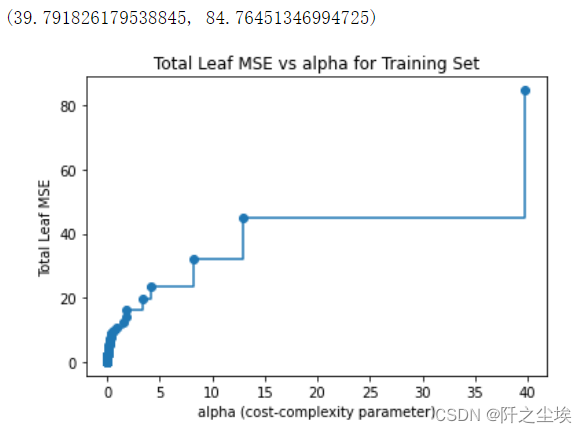

 网格化搜索最优超参数——惩罚系数

param_grid = {'ccp_alpha': path.ccp_alphas} 
kfold = KFold(n_splits=10, shuffle=True, random_state=1)
model = GridSearchCV(DecisionTreeRegressor(random_state=123), param_grid, cv=kfold)
model.fit(X_train, y_train)

model.best_params_

model = model.best_estimator_

model.score(X_test,y_test)

plot_tree(model, feature_names=Boston.feature_names, node_ids=True, rounded=True, precision=2)
plt.tight_layout()
plt.savefig('tree2.png',dpi=900)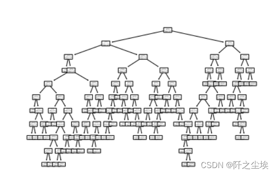

这个树的分支有点多

下面是模型的参数和变量重要性的可视化：

#决策树的深度
model.get_depth()
#叶子节点个数
model.get_n_leaves()
#所有参数
model.get_params()

# Visualize Feature Importance
#变量重要性的可视化
model.feature_importances_
sorted_index = model.feature_importances_.argsort()
X = pd.DataFrame(Boston.data, columns=Boston.feature_names)
plt.barh(range(X.shape[1]), model.feature_importances_[sorted_index])
plt.yticks(np.arange(X.shape[1]), X.columns[sorted_index])
plt.xlabel('Feature Importance')
plt.ylabel('Feature')
plt.title('Decision Tree')
plt.tight_layout()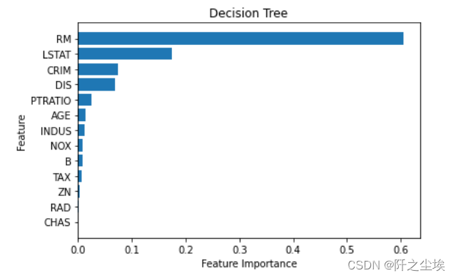

 可以看出对于房价影响最大的是房间数量RM

看预测的拟合值和真实值的对比：

pred = model.predict(X_test)
plt.scatter(pred, y_test, alpha=0.6)
w = np.linspace(min(pred), max(pred), 100)
plt.plot(w, w)
plt.xlabel('pred')
plt.ylabel('y_test')
plt.title('Tree Prediction')

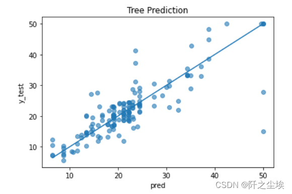还不错

 分类树的Python案例

下面采用银行市场营销的数据，响应变量y为是否贷款，导包读取数据

import numpy as np
import pandas as pd
import matplotlib.pyplot as plt
from sklearn.model_selection import train_test_split
from sklearn.model_selection import KFold, StratifiedKFold
from sklearn.model_selection import GridSearchCV
from sklearn.tree import DecisionTreeRegressor,export_text
from sklearn.tree import DecisionTreeClassifier, plot_tree
from sklearn.datasets import load_boston
from sklearn.metrics import cohen_kappa_score

bank = pd.read_csv('bank-additional.csv', sep=';')
bank.shape

pd.options.display.max_columns = 30 
bank.head()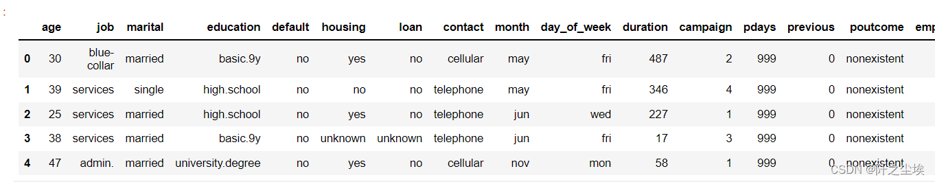

 数据长上面那样子，变量有点多，下面清洗，对分类数据生成虚拟变量后，然后划分训练测试集，开始决策树的拟合。

# Drop 'duration' variable
bank = bank.drop('duration', axis=1)

X_raw = bank.iloc[:, :-1]
X = pd.get_dummies(X_raw)
X.head(2)
#取出y
y = bank.iloc[:, -1]

X_train, X_test, y_train, y_test = train_test_split(X, y, stratify=y, test_size=1000, random_state=1)

# Classification Tree 

model = DecisionTreeClassifier(max_depth=2, random_state=123)
model.fit(X_train, y_train)#拟合
#评价
model.score(X_test, y_test)
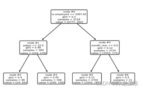
#画决策树
plot_tree(model, feature_names=X.columns, node_ids=True, rounded=True, precision=2)

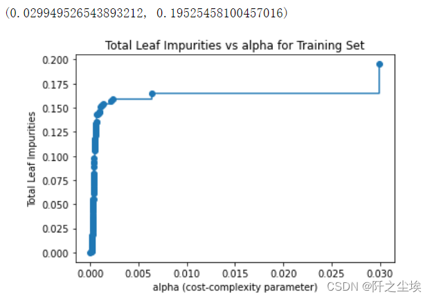
 惩罚系数和损失函数的关系

# Graph total impurities versus ccp_alphas 
model = DecisionTreeClassifier(random_state=123)
path = model.cost_complexity_pruning_path(X_train, y_train)

plt.plot(path.ccp_alphas, path.impurities, marker='o', drawstyle='steps-post')
plt.xlabel('alpha (cost-complexity parameter)')
plt.ylabel('Total Leaf Impurities')
plt.title('Total Leaf Impurities vs alpha for Training Set')

max(path.ccp_alphas),  max(path.impurities)

 网格化搜索最优超参数

param_grid = {'ccp_alpha': path.ccp_alphas}
kfold = StratifiedKFold(n_splits=10, shuffle=True, random_state=1)
model = GridSearchCV(DecisionTreeClassifier(random_state=123), param_grid, cv=kfold)
model.fit(X_train, y_train) 

model.best_params_

model = model.best_estimator_
model.score(X_test, y_test)

plot_tree(model, feature_names=X.columns, node_ids=True, impurity=True, proportion=True, rounded=True, precision=2)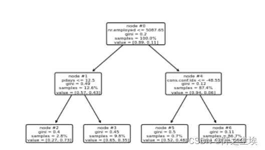    

变量重要性可视化

model.feature_importances_

sorted_index = model.feature_importances_.argsort()
plt.barh(range(X_train.shape[1]), model.feature_importances_[sorted_index])
plt.yticks(np.arange(X_train.shape[1]), X_train.columns[sorted_index])
plt.xlabel('Feature Importance')
plt.ylabel('Feature')
plt.title('Decision Tree')
plt.tight_layout()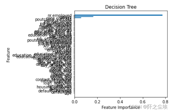

#算混淆矩阵
# Prediction Performance 
pred = model.predict(X_test)
table = pd.crosstab(y_test, pred, rownames=['Actual'], colnames=['Predicted'])
table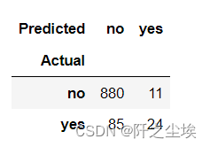

计算混淆矩阵的指标

table = np.array(table)
Accuracy = (table[0, 0] + table[1, 1]) / np.sum(table)
Accuracy

Sensitivity  = table[1, 1] / (table[1, 0] + table[1, 1])
Sensitivity

cohen_kappa_score(y_test, pred)

 采用0.1为分类阈值，计算混淆矩阵和指标

prob = model.predict_proba(X_test)
prob
model.classes_
prob_yes = prob[:, 1]
pred_new = (prob_yes >= 0.1)
pred_new
table = pd.crosstab(y_test, pred_new, rownames=['Actual'], colnames=['Predicted'])
table

table = np.array(table)
Accuracy = (table[0, 0] + table[1, 1]) / np.sum(table)
Accuracy

Sensitivity  = table[1, 1] / (table[1, 0] + table[1, 1])
Sensitivity

使用交叉熵为损失函数，进行网格化搜参进行最优决策树估计

param_grid = {'ccp_alpha': path.ccp_alphas}
kfold = StratifiedKFold(n_splits=10, shuffle=True, random_state=1)
model = GridSearchCV(DecisionTreeClassifier(criterion='entropy', random_state=123), param_grid, cv=kfold)

model.fit(X_train, y_train)     
model.score(X_test, y_test)

pred = model.predict(X_test)
pd.crosstab(y_test, pred, rownames=['Actual'], colnames=['Predicted'])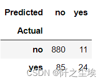

使用鸢尾花数据集两个特征变量进行决策边界的可视化画 

## Decision boundary for iris data
from sklearn.datasets import load_iris
from mlxtend.plotting import plot_decision_regions

X,y = load_iris(return_X_y=True)
X2 = X[:, 2:4]

model = DecisionTreeClassifier(random_state=123)
path = model.cost_complexity_pruning_path(X2, y)
param_grid = {'ccp_alpha': path.ccp_alphas}
kfold = StratifiedKFold(n_splits=10, shuffle=True, random_state=1)
model = GridSearchCV(DecisionTreeClassifier(random_state=123), param_grid, cv=kfold)
model.fit(X2, y)
model.score(X2, y)


plot_decision_regions(X2, y, model)
plt.xlabel('petal_length')
plt.ylabel('petal_width')
plt.title('Decision Boundary for Decision Tree')

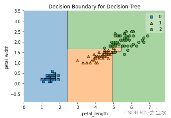可以看出，决策边界都是矩形区域。

最后

以上就是时尚睫毛膏为你收集整理的Python机器学习08——决策树算法的全部内容，希望文章能够帮你解决Python机器学习08——决策树算法所遇到的程序开发问题。

如果觉得靠谱客网站的内容还不错，欢迎将靠谱客网站推荐给程序员好友。