深度学习入门--手写数字识别（Keras）

#导入所需要的包
import keras
from keras.datasets import mnist
from keras.layers import Dense 
from keras.models import Sequential
from keras.optimizers import SGD

#下载数据集
(x_train,y_train),(x_test,y_test) = mnist.load_data()

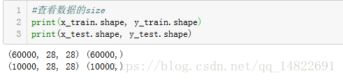
#查看数据的size
print(x_train.shape, y_train.shape)
print(x_test.shape, y_test.shape)

此时输出的结果为：

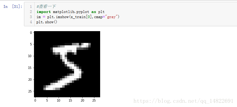
#随机查看一下数据内容
import matplotlib.pyplot as plt
im = plt.imshow(x_train[0],cmap="gray")
plt.show()

输出为：

#向量化图片，将28*28转化成1*784
x_train = x_train.reshape(60000,784)
x_test = x_test.reshape(10000,784)


#数据归一化
x_train = x_train/255
x_test = x_test/255


#将标签值y进行独热编码 keras.utils.to_categorical（）
y_train = keras.utils.to_categorical(y_train,10)
y_test = keras.utils.to_categorical(y_test,10)

#开始构建模型
model = Sequential()
model.add(Dense(512, activation='relu', input_shape=(784,)))
model.add(Dense(256, activation='relu'))
model.add(Dense(10, activation='softmax'))


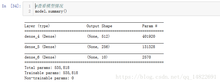
#查看模型情况
model.summary()

输出的模型概况为：

#编译神经网络
model.compile(optimizer=SGD(), loss='categorical_crossentropy', metrics=['accuracy'])

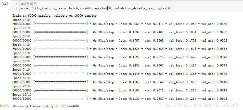
#训练网络
model.fit(x_train, y_train, batch_size=64, epochs=10, validation_data=(x_test, y_test))

执行结果：

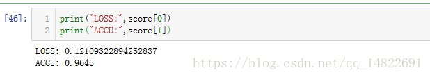
#查看最终结果
score = model.evaluate(x_test, y_test)
print("LOSS:",score[0])
print("ACCU:",score[1])

输出结果为：

完整版程序：

#导入所需要的包
import keras
from keras.datasets import mnist
from keras.layers import Dense 
from keras.models import Sequential
from keras.optimizers import SGD

#下载数据集
(x_train,y_train),(x_test,y_test) = mnist.load_data()

#查看数据的size
#此部分可省略
print(x_train.shape, y_train.shape)
print(x_test.shape, y_test.shape)


#随机查看一下图片
#此部分可省略
import matplotlib.pyplot as plt
im = plt.imshow(x_train[0],cmap="gray")
plt.show()


#向量化图片，将28*28转化成1*784
x_train = x_train.reshape(60000,784)
x_test = x_test.reshape(10000,784)


#数据归一化
x_train = x_train/255
x_test = x_test/255


#将标签值y进行独热编码 keras.utils.to_categorical（）
y_train = keras.utils.to_categorical(y_train,10)
y_test = keras.utils.to_categorical(y_test,10)

#开始构建模型
model = Sequential()
model.add(Dense(512, activation='relu', input_shape=(784,)))
model.add(Dense(256, activation='relu'))
model.add(Dense(10, activation='softmax'))


#查看模型情况
#此部分可省略
model.summary()


#编译神经网络
model.compile(optimizer=SGD(), loss='categorical_crossentropy', metrics=['accuracy'])


#训练网络
model.fit(x_train, y_train, batch_size=64, epochs=10, validation_data=(x_test, y_test))

#查看结果
score = model.evaluate(x_test, y_test)
print("LOSS:",score[0])
print("ACCU:",score[1])

来源：慕课网学习笔记

最后

以上就是缓慢冷风为你收集整理的深度学习入门--手写数字识别（Keras）的全部内容，希望文章能够帮你解决深度学习入门--手写数字识别（Keras）所遇到的程序开发问题。

如果觉得靠谱客网站的内容还不错，欢迎将靠谱客网站推荐给程序员好友。