1. 训练时，分类器记住所有的训练数据；
2. 测试时，每一个测试图像都要和所有的训练图像计算距离，然后选取距离最近的k个图像，最后选取k个图像中出现次数最多的类标签作为输出（预测标签）。

准备工作

为jupyter notebook运行一些准备代码

# 使python2.x也能使用print()
from __future__ import print_function
# 之后需要随机选7张图片
import random
import numpy as np
# 导入数据集
from cs231n.data_utils import load_CIFAR10
# 为画图做准备
import matplotlib.pyplot as plt

# 这是使matplotlib图像出现jupyter notebook里，而不是出现在新窗口的一个小技巧
%matplotlib inline
# 设置画图的默认大小
plt.rcParams['figure.figsize'] = (10.0, 8.0) 
# 最近邻差插值: 像素为正方形
plt.rcParams['image.interpolation'] = 'nearest'
# 使用灰度输出而不是彩色输出
plt.rcParams['image.cmap'] = 'gray'

# 在执行用户代码前，重新装入软件的扩展和模块。autoreload意思是自动重新装入。无参：装入所有模块。
# 修改完.py文件后不需要重新从头运行，只需要重新装载修改过的函数即可
%load_ext autoreload
%autoreload 2

加载CIFAR-10数据

cifar10_dir = 'cs231n/datasets/cifar-10-batches-py'
# 清除变量，以防加载多次（可能导致内存问题）
try:
   del X_train, y_train
   del X_test, y_test
   print('Clear previously loaded data.')
except:
   pass

# 加载数据
X_train, y_train, X_test, y_test = load_CIFAR10(cifar10_dir)
# 输出训练数据和测试数据的大小
print('Training data shape: ', X_train.shape)
# Training data shape:  (50000, 32, 32, 3)
print('Training labels shape: ', y_train.shape)
# Training labels shape:  (50000,)
print('Test data shape: ', X_test.shape)
# Test data shape:  (10000, 32, 32, 3)
print('Test labels shape: ', y_test.shape)
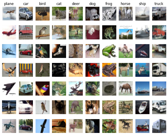
# Test labels shape:  (10000,)

每个类可视化一些图像

# 类标签
classes = ['plane', 'car', 'bird', 'cat', 'deer', 'dog', 'frog', 'horse', 'ship', 'truck']
# 类的个数（10）
num_classes = len(classes)
# 每个类的样例
samples_per_class = 7
# y是索引值（0-9），cls是名字（'plane'等）
for y, cls in enumerate(classes):
    # 在训练数据标签y_train中记录标签为y的下标（y_train中存放的是数字）
    idxs = np.flatnonzero(y_train == y)
    # 同一标签的图片中随机选7张（记录的是下标）
    idxs = np.random.choice(idxs, samples_per_class, replace=False)
    # i代表该类选出来的第i张图片，idx是该图片在训练数据集里的下标
    for i, idx in enumerate(idxs):
        # 计算图片所在的位置
        plt_idx = i * num_classes + y + 1
        # 总共是7行10列的图片
        plt.subplot(samples_per_class, num_classes, plt_idx)
        plt.imshow(X_train[idx].astype('uint8'))
        # 不显示坐标轴
        plt.axis('off')
        if i == 0:
            # 第一行图片上输出类别标签
            plt.title(cls)
plt.show()

可视化结果：

为了更高效地执行代码，我们只取样部分数据。选取5000张测试图片，500张测试图片。

num_training = 5000
mask = list(range(num_training))
X_train = X_train[mask]
y_train = y_train[mask]

num_test = 500
mask = list(range(num_test))
X_test = X_test[mask]
y_test = y_test[mask]

把每张32*32*3的图片变为1*3072的行向量

X_train = np.reshape(X_train, (X_train.shape[0], -1))
X_test = np.reshape(X_test, (X_test.shape[0], -1))
print(X_train.shape, X_test.shape)
# (5000, 3072) (500, 3072)

KNN

创建一个KNN分类器实例

from cs231n.classifiers import KNearestNeighbor
classifier = KNearestNeighbor()
# 训练就是记住所有图片和标签
classifier.train(X_train, y_train)

训练函数：

def train(self, X, y):
  # X[i]是图片，y[i]是X[i]的标签
  self.X_train = X
  self.y_train = y

使用两层循环计算测试数据集和训练数据集的L2距离

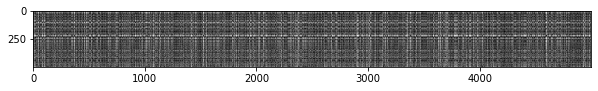
dists = classifier.compute_distances_two_loops(X_test)
print(dists.shape)
# (500, 5000)（测试数据集个数，训练数据集个数）
# 对距离矩阵可视化，不进行插值
plt.imshow(dists, interpolation='none')
plt.show()

亮的地方代表距离比较远，暗的地方代表距离比较近

1. 比较亮的横线代表，该测试图像和训练数据集里的所有图像都不像
2. 比较亮的列代表，该训练数据集里的图片和所有测试图片都不像
   

两重循环的距离函数：

def compute_distances_two_loops(self, X):
  # X是测试数据集
  num_test = X.shape[0]
  num_train = self.X_train.shape[0]
  # dists[i,j]表示第i个测试数据和第j个训练数据的L2距离
  dists = np.zeros((num_test, num_train))
  for i in range(num_test):
    for j in range(num_train):
      dis = (X[i]-self.X_train[j])**2
      # dis是向量，np.sum是求向量的和，然后开平方
      dists[i,j] = np.sqrt(np.sum(dis))
  return dists

使用最临近（k=1）预测标签，应该得到27%左右的准确率

y_test_pred = classifier.predict_labels(dists, k=1)
# 计算准确率
num_correct = np.sum(y_test_pred == y_test)
accuracy = float(num_correct) / num_test
print('Got %d / %d correct => accuracy: %f' % (num_correct, num_test, accuracy))

预测函数：

def predict_labels(self, dists, k=1):
  num_test = dists.shape[0]
  # 预测num_test个数据的标签
  y_pred = np.zeros(num_test)
  for i in range(num_test):
    # 储存k个与测试数据X[i]距离最近的数据的标签
    closest_y = []
    # argsort函数返回的是数组值从小到大排序的下标    
    # >>> x = np.array([3, 1, 2])
    # >>> np.argsort(x)
    # array([1, 2, 0])
    sort_dist = np.argsort(dists[i])
    # 取前k个下标的标签，即距离最近的k个数据的标签    
    # >>> x[np.argsort(x)] #通过索引值排序后的数组
    # array([1, 2, 3])
    closest_y = self.y_train[sort_dist[:k]]
    # 把预测标签保存在y_pred[i]，如果标签出现的数量相同，选择最小的标签
    # 假设k=8时closest_y结果如下。closest_y中最大的数为10——10个类别，因此bin的数量为11，那么它的索引值为0->10
    # closest_y = np.array([2, 1, 1, 3, 10, 3, 7, 6])
    # 标签0出现了0次，标签1出现了2次......标签8出现了0次......
    # np.bincount(closest_y)
    # 因此，输出结果为：array([0, 2, 1, 2, 0, 0, 1, 1, 0, 0, 1])
    # >>> np.argmax(np.bincount(closest_y))
    # 1（出现次数最多的标签为1和3，但是1比3小，所以预测的结果是1——飞机）
    y_pred[i] = np.argmax(np.bincount(closest_y))
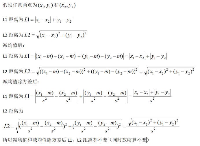
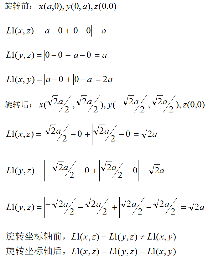
  return y_pred

我们还可以使用L1距离来计算KNN。下列表达中L1距离不会变的是：

• 数据减均值
• 数据减均值后除方差
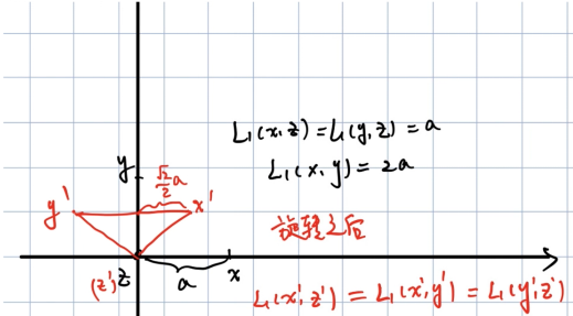
• 旋转坐标轴
• 以上都对

减均值和减均值除方差的情况：

旋转坐标轴的情况（橙色的是旋转后的）：


k=5的时候，准确率应该比刚才稍微好一点

y_test_pred = classifier.predict_labels(dists, k=5)
num_correct = np.sum(y_test_pred == y_test)
accuracy = float(num_correct) / num_test
print('Got %d / %d correct => accuracy: %f' % (num_correct, num_test, accuracy))

使用一重循环计算距离矩阵：

dists_one = classifier.compute_distances_one_loop(X_test)
# 计算两个矩阵差的二范数
difference = np.linalg.norm(dists - dists_one, ord='fro')
print('Difference was: %f' % (difference, ))
# Difference was: 0.000000（使用两重循环和一重循环计算出来的距离是一样的）
if difference < 0.001:
    print('Good! The distance matrices are the same')
else:
    print('Uh-oh! The distance matrices are different')
# Good! The distance matrices are the same

一重循环计算L2距离的函数：

def compute_distances_one_loop(self, X):
  m_test = X.shape[0]
  num_train = self.X_train.shape[0]
  dists = np.zeros((num_test, num_train))
  for i in range(num_test):
    # self.X_train是(5000,3072)的矩阵，X[i]是(1,3072)的行向量。会把X[i]复制4999份，把X[i]扩充成(5000,3072)的矩阵，所以时间、空间花费都很大。
    dif = self.X_train - X[i]
    dist = np.sum(dif**2,axis = 1)#沿着行求和
    dists[i,:] = np.sqrt(dist)
  return dists

不使用循环计算距离矩阵：

dists_two = classifier.compute_distances_no_loops(X_test)
difference = np.linalg.norm(dists - dists_two, ord='fro')
# Difference was: 0.000000（使用两重循环和不使用循环计算出来的距离是一样的）
print('Difference was: %f' % (difference, ))
if difference < 0.001:
    print('Good! The distance matrices are the same')
else:
    print('Uh-oh! The distance matrices are different')
# Good! The distance matrices are the same

不使用循环计算L2距离：

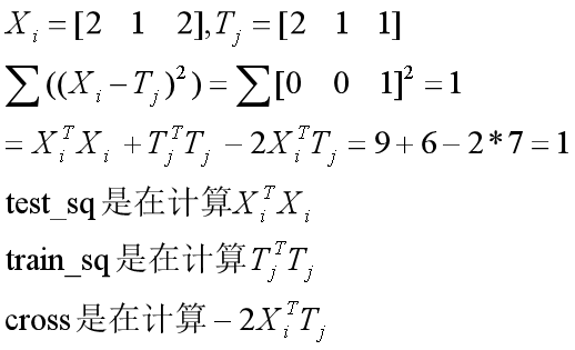
def compute_distances_no_loops(self, X):
  m_test = X.shape[0]
  num_train = self.X_train.shape[0]
  dists = np.zeros((num_test, num_train)) 
  # (x-y)^2=x^2+y^2-2xy
  test_sq = np.sum(X**2,axis=1)# x^2,(500,1)
  train_sq = np.sum(self.X_train**2,axis=1)# y^2,(5000,1)
  cross = np.multiply(np.dot(X,self.X_train.T),-2)# -2xy,(500,5000)
  dists = np.add(cross,test_sq)
  dists = np.add(dists,train_sq)
  dists = np.sqrt(dists)
  return dists

比较一下哪种循环更快：

def time_function(f, *args):
    # 计算函数f运行所需时间，后面输入的是函数f的参数
    import time
    # 记录开始时间
    tic = time.time()
    f(*args)
    # 记录结束时间
    toc = time.time()
    return toc - tic

# 计算两重循环所需时间
two_loop_time = time_function(classifier.compute_distances_two_loops, X_test)
print('Two loop version took %f seconds' % two_loop_time)
# Two loop version took 43.185944 seconds

# 计算一重循环所需时间
one_loop_time = time_function(classifier.compute_distances_one_loop, X_test)
print('One loop version took %f seconds' % one_loop_time)
# One loop version took 96.849304 seconds

# 计算不需要循环所需的时间
no_loop_time = time_function(classifier.compute_distances_no_loops, X_test)
print('No loop version took %f seconds' % no_loop_time)
# No loop version took 0.343081 seconds

一重循环要开辟更多的空间，所以运算速度比较慢。

交叉验证

计算不同k值的准确率

# 5折交叉验证
num_folds = 5
k_choices = [1, 3, 5, 8, 10, 12, 15, 20, 50, 100]
X_train_folds = []
y_train_folds = []
y_train_ = y_train.reshape(-1, 1)#变成1列
# 分成5个小训练数据集
X_train_folds = np.array_split(X_train, num_folds)
y_train_folds = np.array_split(y_train, num_folds)
# 保存准确率
k_to_accuracies = {}
for k in k_choices:
    accuracies = []
    for i in range(num_folds):
        # 把第i个小训练数据集当作验证集
        X_test_cv = X_train_folds[i]
        # 除第i个以外的训练集作为训练集
        X_train_cv = np.vstack(X_train_folds[:i] + X_train_folds[i+1:])
        
        y_test_cv = y_train_folds[i]
        y_train_cv = np.hstack(y_train_folds[:i]+y_train_folds[i+1:])
        
        classifier.train(X_train_cv, y_train_cv)
        dists_cv = classifier.compute_distances_no_loops(X_test_cv)
        
        y_test_pred = classifier.predict_labels(dists_cv, k)
        num_correct = np.sum(y_test_pred == y_test_cv)
        accuracies.append(float(num_correct) * num_folds / num_training)
    k_to_accuracies[k] = accuracies
for k in sorted(k_to_accuracies):
    for accuracy in k_to_accuracies[k]:
        print('k = %d, accuracy = %f' % (k, accuracy))

画出交叉验证的图

for k in k_choices:
    accuracies = k_to_accuracies[k]
    # [k] * 5 = [k,k,k,k,k],就是画一列点
    plt.scatter([k] * len(accuracies), accuracies)
# 计算准确率的均值
accuracies_mean = np.array([np.mean(v) for k,v in sorted(k_to_accuracies.items())])
# 计算准确率的方差
accuracies_std = np.array([np.std(v) for k,v in sorted(k_to_accuracies.items())])
# plt.errorbar()函数用于表现有一定置信区间的带误差数据，就是蓝色的竖线和均值折线
plt.errorbar(k_choices, accuracies_mean, yerr=accuracies_std)
plt.title('Cross-validation on k')
plt.xlabel('k')
plt.ylabel('Cross-validation accuracy')
plt.show()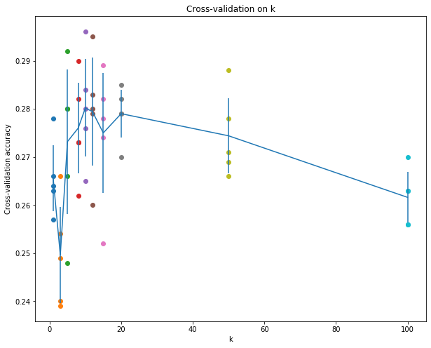

通过图片选择效果最好的k值（10），并计算它的准确率（应该大于28%）

best_k = 10
classifier = KNearestNeighbor()
classifier.train(X_train, y_train)
y_test_pred = classifier.predict(X_test, k=best_k)
num_correct = np.sum(y_test_pred == y_test)
accuracy = float(num_correct) / num_test
print('Got %d / %d correct => accuracy: %f' % (num_correct, num_test, accuracy))

下列哪些表达正确：

• 训练数据在k=1时的准确率总是比k=5时要好
• 测试数据在k=1时的准确率总是比k=5时要好
• KNN分类器的决策边界是线性的
• 预测一个测试样例的标签所花费的时间随着训练数据集的增大而增大
• 以上都对

1. 训练数据在k=1时的预测准确率为100%（因为有相同的图片，距离为0）；而k=5时可能会被别的图片误导
2. 这是不一定的，有可能更好也有可能更差
3. KNN需要选择距离最近的k个标签所以不是线性的
4. 因为每一个测试样例都要和所有的训练数据计算距离，而且在选择距离最近的k个标签所花的时间也和标签的总数（训练数据的个数）有关。

最后

以上就是幸福日记本为你收集整理的【深度之眼cs231n第七期】笔记（四）准备工作KNN交叉验证的全部内容，希望文章能够帮你解决【深度之眼cs231n第七期】笔记（四）准备工作KNN交叉验证所遇到的程序开发问题。

如果觉得靠谱客网站的内容还不错，欢迎将靠谱客网站推荐给程序员好友。