前言

          前段时间学习了深度学习入门课程斯坦福CS231n，巩固和理解课程的最佳方式就是完成课后代码作业。在这里记录下本人对作业的思考和解析，以供大家参考。

          关于CS231n学习笔记翻译，强烈推荐 知乎专栏 。

          配合笔记看视频，再完成作业，非常有效。

一、准备工作

1、作业Assignment1下载

        链接：https://pan.baidu.com/s/11tDkdBRy5ndwkKue_1vMuw 密码：jvgk

2、环境Anaconda2安装

         完成作业需要Python以及许多相关科学计算环境，建议大家直接安装Anaconda2，能够快速方便的配置，直接上手写作业。代码是Python 2.x版本，故选择Anaconda2-4.2.0-Windows-x86_64.exe，否则可能出现某些函数不兼容，造成不必要的麻烦。

3、数据集CIFAR-10下载

         简单介绍一下，CIFAR-10是一个只有10类图片的彩色图片数据库，共6w张32*32像素大小的图片，其中5w张是训练图片，1w张是测试图片，所有图片均已标记。

        选择CIFAR10 python version下载，解压后将数据放在cs231n/datasets目录下。

4、验证WebSockets是否可用

        作业在Ipython Notebook内完成，需要支持WebSockets。打开下述网页，若显示“WORK FOR YOU”，表示可用。

         测试链接：http://websocketstest.com/

        

         出现以上字样即可。

        若无法使用，需要翻墙。网上可用VPN有很多，大家可以搜索一下。

        至此准备工作全部完成，可以开始写作业啦。

二、作业解析

1、连接服务器

         如图所示，打开cmd，在[your path]/assignment1/目录下输入Ipython notebook 或者 Jupyter notebook，回车。

       

        更多Ipython notebook教程可参考 这里 。

        注意：一定要在目录下打开，否则后面会出现找不到包的情况。

                    退出的话输入ctrl+c，等待关闭即可。

       成功连上服务器后，你将在浏览器下看到如下界面：

      

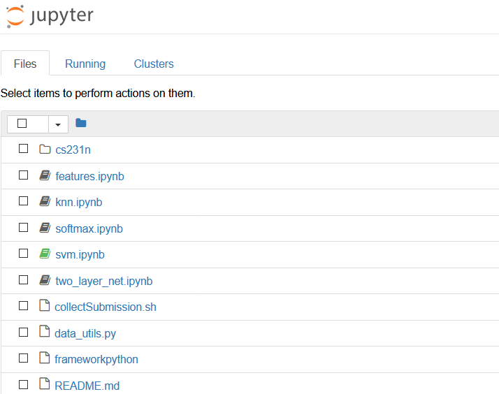
       这次的作业就需要在knn.ipynb下完成。

2、运行代码

        选中代码块，ctrl+enter或shift+enter运行，区别是shift+enter会自动跳转到下一部分。页面右上角的圆圈表示运行状态，空心表示结束，实心表示正在运行。

                                                                                             

          下面对各部分代码进行补充和运行。

           kNN分类器包括两个部分：

•     在训练的时候，分类器载入数据并仅仅记住他们（不做其他处理）

•     在测试的时候，分类器依靠对测试图片和训练图片做对比，并且选出k个最相似的标签

•     另外，k是依靠交叉验证确定的

         在这个作业中，我们将实现这些步骤并且理解基本的图像分类过程，理解交叉验证，并且学会写高效的向量化代码。

3、代码解析

3.1  一些基本的初始化

 # Run some setup code for this notebook.
importrandom
importnumpy as np
fromcs231n.data_utils import load_CIFAR10
importmatplotlib.pyplot as plt

from__future__ import print_function
 

#This is a bit of magic to make matplotlib figures appear inline in the notebook
#rather than in a new window.
%matplotlibinline
plt.rcParams['figure.figsize']= (10.0, 8.0) # set default size of plots
plt.rcParams['image.interpolation']= 'nearest'
plt.rcParams['image.cmap']= 'gray'

#Some more magic so that the notebook will reload external python modules;
#see http://stackoverflow.com/questions/1907993/autoreload-of-modules-in-ipython
%load_extautoreload
%autoreload2

           一些初始化代码，载入必要的包，保证图像输出在网页中而不新建窗口。

3.2 载入数据

 # Load the raw CIFAR-10 data.
cifar10_dir= 'cs231n/datasets/cifar-10-batches-py'
X_train,y_train, X_test, y_test = load_CIFAR10(cifar10_dir)

#As a sanity check, we print out the size of the training and test data.
print('Trainingdata shape: ', X_train.shape)
print('Traininglabels shape: ', y_train.shape)
print('Testdata shape: ', X_test.shape)
print('Testlabels shape: ', y_test.shape)

   载入CIFAR-10数据。输出数据格式：

           

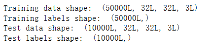
   由于是彩图3通道，故大小为32*32*3.

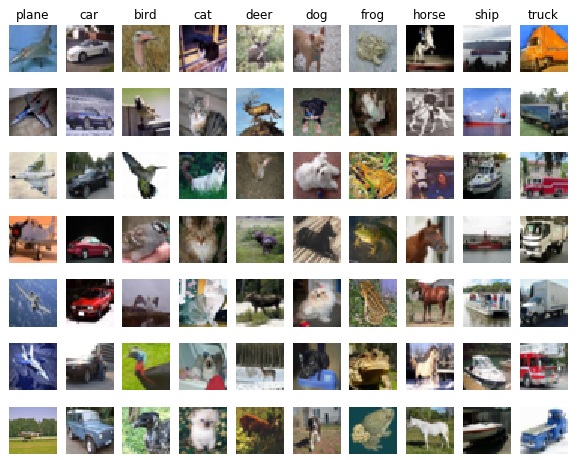
3.3  展示部分训练图

 # Visualize some examples fromthe dataset.
#We show a few examples of training images from each class.
classes= ['plane', 'car', 'bird', 'cat', 'deer', 'dog', 'frog', 'horse', 'ship','truck']
num_classes= len(classes)
samples_per_class= 7
fory, cls in enumerate(classes):
    idxs = np.flatnonzero(y_train == y)
    idxs = np.random.choice(idxs,samples_per_class, replace=False)
    for i, idx in enumerate(idxs):
        plt_idx = i * num_classes + y + 1
        plt.subplot(samples_per_class,num_classes, plt_idx)
        plt.imshow(X_train[idx].astype('uint8'))
        plt.axis('off')

        if i == 0:
            plt.title(cls)
plt.show()

       从每一类中展示7张训练图片。结果如下：

    

3.4    取样数据

#Subsample the data for more efficient code execution in this exercise
num_training= 5000
mask= list(range(num_training))
X_train= X_train[mask]
y_train= y_train[mask]
 
num_test= 500
mask= list(range(num_test))
X_test= X_test[mask]
y_test= y_test[mask]

          在练习中，为了更高效地执行代码，我们只取样部分数据。选取5000张测试图片，500张测试图片。

3.5  数据变形

#Reshape the image data into rows
X_train= np.reshape(X_train, (X_train.shape[0], -1))
X_test= np.reshape(X_test, (X_test.shape[0], -1))

print(X_train.shape,X_test.shape)

      将图片转化为行向量，所有图片组成二维矩阵。32*32*3=3072.

     故结果如下：

(5000L,3072L) (500L, 3072L)

3.6  载入函数

fromcs231n.classifiers import KNearestNeighbor
#Create a kNN classifier instance.
#Remember that training a kNN classifier is a noop:
#the Classifier simply remembers the data and does no further processing
classifier= KNearestNeighbor()
classifier.train(X_train,y_train)

 载入KnearestNeighbour包，创建KNearestNeighbor类的对象classifier，调用train()函数。

3.7   二重循环计算距离矩阵

        现在我们开始计算代表测试图片和训练图片之间距离的矩阵。如果有Ntr张训练数据，Nte张测试数据，那么应该得到Nte*Ntr的距离矩阵，其中(i,j)表示第 i 张测试图距离第 j 张训练图片的距离。

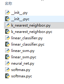
       所以，我们需要实现的cs231n/classifiers/k_nearest_neighbor.py目录下的函数compute_distances_two_loops()，使用了二重循环。

defcompute_distances_two_loops(self, X):
   """
   Compute the distance between each test point in X and each trainingpoint
   in self.X_train using a nested loop over both the training data and the
   test data.
 

   Inputs:
   - X: A numpy array of shape (num_test, D) containing test data.

   Returns:
   - dists: A numpy array of shape (num_test, num_train) where dists[i, j]
      is the Euclidean distance between the ithtest point and the jth training
      point.
   """

   num_test = X.shape[0]
   num_train = self.X_train.shape[0]
   dists = np.zeros((num_test, num_train)) #500*5000
   for i in xrange(num_test):
      for j in xrange(num_train):
         dists[i,j] = np.sqrt(np.sum(np.square(self.X_train[j,:]- X[i,:])))
       #####################################################################
        # TODO:                                                            #
        # Compute the L2 distance between the ithtest point and the jth    #
        # training point, and store the resultin dists[i, j]. You should   #
        # not use a loop over dimension.                                   #
       #####################################################################
        #pass
       #####################################################################
        #                       END OF YOUR CODE                            #
        #####################################################################
   return dists

         使用的是L2距离，注意 i 和 j 分别代表测试集和训练集。

3.8 测试距离矩阵

#Open cs231n/classifiers/k_nearest_neighbor.py and implement
#compute_distances_two_loops.

#Test your implementation:
dists= classifier.compute_distances_two_loops(X_test)
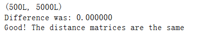
print(dists.shape)

 调用刚刚写好的函数，打印距离矩阵的大小：

 (500L, 5000L)

#We can visualize the distance matrix: each row is a single test example and
#its distances to training examples
plt.imshow(dists,interpolation='none')
plt.show()

   将距离矩阵可视化。每一行表示测试样例距所有训练图片的距离。

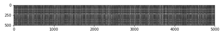
      如上图所示，纵坐标表示500张测试图片，横坐标表示5000张训练图片。越黑表示距离越接近，越亮表示距离越远。

3.9  预测测试图片的标签

         实现预测函数predict_labels()，在cs231n/classifiers/k_nearest_neighbor.py目录下。根据3.7~3.8算出的dists距离矩阵，选出离测试图片最近的k张训练图，投票选出最可能的预测结果。若k=1，就选出距离最近的一张训练图，将该图的标签作为测试图的标签。

def predict_labels(self, dists, k=1):

    """
    Given a matrix of distances between testpoints and training points,
    predict a label for each test point.

    Inputs:
    - dists: A numpy array of shape (num_test,num_train) where dists[i, j]
      gives the distance betwen the ith testpoint and the jth training point.
 
    Returns:
    - y: A numpy array of shape (num_test,)containing predicted labels for the
      test data, where y[i] is the predictedlabel for the test point X[i]. 
    """
    num_test = dists.shape[0]
    y_pred = np.zeros(num_test) #500*1
    for i in xrange(num_test):
      # A list of length k storing the labelsof the k nearest neighbors to
      # the ith test point.
      closest_y = []
     #########################################################################
      # TODO:                                                                #
      # Use the distance matrix to find the knearest neighbors of the ith    #
      # testing point, and use self.y_train tofind the labels of these       #
      # neighbors. Store these labels inclosest_y.                           #
      # Hint: Look up the functionnumpy.argsort.                             #
     #########################################################################

      closest_y = np.argsort(dists[i,:]) # i'm socool
      #pass
     #########################################################################
      # TODO:                                                                #
      # Now that you have found the labels ofthe k nearest neighbors, you    #
      # need to find the most common label inthe list closest_y of labels.   #
      # Store this label in y_pred[i]. Breakties by choosing the smaller     #
      # label.                                                               #
     #########################################################################

      y_pred[i] =np.argmax(np.bincount(self.y_train[closest_y[:k]]))

      #pass
      #########################################################################
      #                           END OF YOURCODE                             #
     #########################################################################
    return y_pred

           对所有的测试图片遍历，将dists[]矩阵按行排序（由大到小），索引放于closet_y向量中。对cloest_y中前k个向量进行计数np.bincount()，最终用np.argmax()得到票数最多的下标，作为最终的标签y_pred[i]。

         举个例子：

        假如cloest_y向量中排名前五的数字分别为[1,1,1,3,2]，那么np.bincount()将会返回索引在该数组内出现的次数：

         array([0, 3, 1, 1])

        因为[1,1,1,3,2]中最大数字为3，故bincount()结果有4个数字，索引值为0~3.数组表示0出现0次，1出现3次，2出现1次，3出现1次。这时候取最大值下标np.argmax()，正好得到索引值1，就是我们希望的结果。

3.10  运行预测代码

# Now implement the function predict_labels and run the code below:
# We use k = 1 (which is Nearest Neighbor).
y_test_pred = classifier.predict_labels(dists, k=1)
# Compute and print the fraction of correctly predicted examples
num_correct = np.sum(y_test_pred == y_test)
accuracy = float(num_correct) / num_test
print('Got %d / %d correct => accuracy: %f' % (num_correct, num_test, accuracy))

结果如下：

Got 137/500 correct => accuracy: 0.274000

3.11 测试k=5的情况

y_test_pred = classifier.predict_labels(dists, k=5)
num_correct = np.sum(y_test_pred == y_test)
accuracy = float(num_correct) / num_test
print('Got %d / %d correct => accuracy: %f' % (num_correct, num_test, accuracy)) 

   结果如下：

Got 139/500 correct => accuracy: 0.278000

   比起刚才的27.4%，准确度有了些微的提升。

3.12  半向量化代码

def compute_distances_one_loop(self, X):

    """
    Compute the distance between each test point in X and each training point
    in self.X_train using a single loop over the test data.

    Input / Output: Same as compute_distances_two_loops
    """
    num_test = X.shape[0]
    num_train = self.X_train.shape[0]
    dists = np.zeros((num_test, num_train))
    for i in xrange(num_test):
      #######################################################################
      # TODO:                                                               #
      # Compute the L2 distance between the ith test point and all training #
      # points, and store the result in dists[i, :].                        #
      #######################################################################
      dists[i,:] = np.sqrt(np.sum(np.square(self.X_train - X[i,:]),axis = 1))
      #pass
      #######################################################################
      #                         END OF YOUR CODE                            #
      #######################################################################
    return dist

       和双重循环的区别在于，单层循环只遍历了测试图片，对训练图片的遍历采用了向量化代码完成。axis=1表示沿着水平方向累加。这是因为要对某张测试图片计算他距离每张训练图片的距离。

3.13  测试半向量化代码

 # Now lets speed up distance matrix computation by using partial vectorization
# with one loop. Implement the function compute_distances_one_loop and run the
# code below:
dists_one = classifier.compute_distances_one_loop(X_test)
print(dists_one.shape)
# To ensure that our vectorized implementation is correct, we make sure that it
# agrees with the naive implementation. There are many ways to decide whether
# two matrices are similar; one of the simplest is the Frobenius norm. In case
# you haven't seen it before, the Frobenius norm of two matrices is the square
# root of the squared sum of differences of all elements; in other words, reshape
# the matrices into vectors and compute the Euclidean distance between them.
difference = np.linalg.norm(dists - dists_one, ord='fro')
print('Difference was: %f' % (difference, ))
if difference < 0.001:
    print('Good! The distance matrices are the same')
else:
    print('Uh-oh! The distance matrices are different')

  证明我们的半向量化代码是正确的。

3.14  向量化代码

        这一部分是最核心、最难以理解，也是最高效的代码。要求不能包含任何循环，依靠numpy提供的广播机制来计算矩阵。

        首先考虑两个需要计算的矩阵。一个包含测试图片的矩阵X，大小是500*3072，表示有500张测试图，每一行代表图片的像素情况；另一个是包含训练图片的矩阵X_train，有5000张图片，故大小为5000*3072。需要做的就是将测试矩阵的每一行和训练矩阵的每一行做L2距离计算，结果存在dists矩阵（500*5000）中。

        考虑L2距离的计算公式：

            

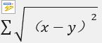
        对求和符号内部公式展开得：x^2 + y ^2 – 2*x*y。

        所谓广播机制，是指两个矩阵在每一维上维度相等或者其中一个矩阵的维度是1的情况下，较小的矩阵将自动扩展为较大矩阵同样的大小。举例如下：

        矩阵a = [[1,2,3]

                       [1,2,3]

                       [1,2,3]] 

               b =  [1 1 1]

         a矩阵维度为3*3，b矩阵维度为1*3.由于a和b在列上维度相同，b矩阵在行上维度为1。故a = a+b的结果将为：

               a = [[2,3,4]

                      [2,3,4]

                      [2,3,4]]

         相当于将b矩阵按行广播，变为[[1,1,1][1,1,1][1,1,1]]了。

         更多广播机制的内容参见 这里 。

def compute_distances_no_loops(self, X):
    """
    Compute the distance between each test point in X and each training point
    in self.X_train using no explicit loops.

    Input / Output: Same as compute_distances_two_loops
    """
    num_test = X.shape[0]
    num_train = self.X_train.shape[0]
    dists = np.zeros((num_test, num_train)) 
    #########################################################################
    # TODO:                                                                 #
    # Compute the L2 distance between all test points and all training      #
    # points without using any explicit loops, and store the result in      #
    # dists.                                                                #
    #                                                                       #
    # You should implement this function using only basic array operations; #
    # in particular you should not use functions from scipy.                #
    #                                                                       #
    # HINT: Try to formulate the l2 distance using matrix multiplication    #
    #       and two broadcast sums.                                         #
    #########################################################################
    dists += np.sum(self.X_train ** 2, axis=1).reshape(1, num_train) #1*5000，第一次广播
    dists += np.sum(X ** 2, axis=1).reshape(num_test,1) #500*1，第二次广播
    dists -= 2 * np.dot(X, self.X_train.T) #500*5000
    dists = np.sqrt(dists)
    #pass
    #########################################################################
    #                         END OF YOUR CODE                              #
    #########################################################################
    return dists

3.15 测试向量化代码

# Now implement the fully vectorized version inside compute_distances_no_loops
# and run the code
dists_two = classifier.compute_distances_no_loops(X_test)

# check that the distance matrix agrees with the one we computed before:
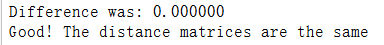
difference = np.linalg.norm(dists - dists_two, ord='fro')
print('Difference was: %f' % (difference, ))
if difference < 0.001:
    print('Good! The distance matrices are the same')
else:
    print('Uh-oh! The distance matrices are different')

运行结果：

3.16 比较各函数效果

# Let's compare how fast the implementations are
def time_function(f, *args):
    """
    Call a function f with args and return the time (in seconds) that it took to execute.
    """
    import time
    tic = time.time()
    f(*args)
    toc = time.time()
    return toc - tic

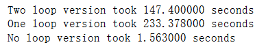
two_loop_time = time_function(classifier.compute_distances_two_loops, X_test)
print('Two loop version took %f seconds' % two_loop_time)

one_loop_time = time_function(classifier.compute_distances_one_loop, X_test)
print('One loop version took %f seconds' % one_loop_time)

no_loop_time = time_function(classifier.compute_distances_no_loops, X_test)
print('No loop version took %f seconds' % no_loop_time)

# you should see significantly faster performance with the fully vectorized implementation

      我们在3.14实现了向量化函数，在3.12实现了半向量化函数，在3.7实现了无向量化函数。对他们用时分别测试。结果如下：

3.17  交叉验证

num_folds = 5
k_choices = [1, 3, 5, 8, 10, 12, 15, 20, 50, 100]

X_train_folds = []
y_train_folds = []
################################################################################
# TODO:                                                                        #
# Split up the training data into folds. After splitting, X_train_folds and    #
# y_train_folds should each be lists of length num_folds, where                #
# y_train_folds[i] is the label vector for the points in X_train_folds[i].     #
# Hint: Look up the numpy array_split function.                                #
################################################################################
# split self.X_train to 5 folds
avg_size = int(X_train.shape[0] / num_folds) # will abandon the rest if not divided evenly.
for i in range(num_folds):
    X_train_folds.append(X_train[i * avg_size : (i+1) * avg_size])
    y_train_folds.append(y_train[i * avg_size : (i+1) * avg_size])

pass
################################################################################
#                                 END OF YOUR CODE                             #
################################################################################

# A dictionary holding the accuracies for different values of k that we find
# when running cross-validation. After running cross-validation,
# k_to_accuracies[k] should be a list of length num_folds giving the different
# accuracy values that we found when using that value of k.
k_to_accuracies = {}


################################################################################
# TODO:                                                                        #
# Perform k-fold cross validation to find the best value of k. For each        #
# possible value of k, run the k-nearest-neighbor algorithm num_folds times,   #
# where in each case you use all but one of the folds as training data and the #
# last fold as a validation set. Store the accuracies for all fold and all     #
# values of k in the k_to_accuracies dictionary.                               #
################################################################################
for k in k_choices:
    accuracies = []
    print(k)
    for i in range(num_folds):
        X_train_cv = np.vstack(X_train_folds[0:i] + X_train_folds[i+1:])
        y_train_cv = np.hstack(y_train_folds[0:i] + y_train_folds[i+1:])
        X_valid_cv = X_train_folds[i]
        y_valid_cv = y_train_folds[i]
        
        classifier.train(X_train_cv, y_train_cv)
        dists = classifier.compute_distances_no_loops(X_valid_cv)
        accuracy = float(np.sum(classifier.predict_labels(dists, k) == y_valid_cv)) / y_valid_cv.shape[0]
        accuracies.append(accuracy)
    k_to_accuracies[k] = accuracies
pass
################################################################################
#                                 END OF YOUR CODE                             #
################################################################################

# Print out the computed accuracies
for k in sorted(k_to_accuracies):
    for accuracy in k_to_accuracies[k]:
        print('k = %d, accuracy = %f' % (k, accuracy))

       这部分代码不难理解，主要将训练代码分为5部分，其中一部分作为验证集，来不断改变k值，寻找最优解。其中np.vstack()表示沿着竖直方向将矩阵堆叠，np.hstack()表示沿水平方向堆叠矩阵。运行结果：

1
3
5
8
10
12
15
20
50
100
k = 1, accuracy = 0.263000
k = 1, accuracy = 0.257000
k = 1, accuracy = 0.264000
k = 1, accuracy = 0.278000
k = 1, accuracy = 0.266000
k = 3, accuracy = 0.239000
k = 3, accuracy = 0.249000
k = 3, accuracy = 0.240000
k = 3, accuracy = 0.266000
k = 3, accuracy = 0.254000
k = 5, accuracy = 0.248000
k = 5, accuracy = 0.266000
k = 5, accuracy = 0.280000
k = 5, accuracy = 0.292000
k = 5, accuracy = 0.280000
k = 8, accuracy = 0.262000
k = 8, accuracy = 0.282000
k = 8, accuracy = 0.273000
k = 8, accuracy = 0.290000
k = 8, accuracy = 0.273000
k = 10, accuracy = 0.265000
k = 10, accuracy = 0.296000
k = 10, accuracy = 0.276000
k = 10, accuracy = 0.284000
k = 10, accuracy = 0.280000
k = 12, accuracy = 0.260000
k = 12, accuracy = 0.295000
k = 12, accuracy = 0.279000
k = 12, accuracy = 0.283000
k = 12, accuracy = 0.280000
k = 15, accuracy = 0.252000
k = 15, accuracy = 0.289000
k = 15, accuracy = 0.278000
k = 15, accuracy = 0.282000
k = 15, accuracy = 0.274000
k = 20, accuracy = 0.270000
k = 20, accuracy = 0.279000
k = 20, accuracy = 0.279000
k = 20, accuracy = 0.282000
k = 20, accuracy = 0.285000
k = 50, accuracy = 0.271000
k = 50, accuracy = 0.288000
k = 50, accuracy = 0.278000
k = 50, accuracy = 0.269000
k = 50, accuracy = 0.266000
k = 100, accuracy = 0.256000
k = 100, accuracy = 0.270000
k = 100, accuracy = 0.263000
k = 100, accuracy = 0.256000
k = 100, accuracy = 0.263000

3.18 结果可视化

# plot the raw observations
for k in k_choices:
    accuracies = k_to_accuracies[k]
    plt.scatter([k] * len(accuracies), accuracies)

# plot the trend line with error bars that correspond to standard deviation
accuracies_mean = np.array([np.mean(v) for k,v in sorted(k_to_accuracies.items())])
accuracies_std = np.array([np.std(v) for k,v in sorted(k_to_accuracies.items())])
plt.errorbar(k_choices, accuracies_mean, yerr=accuracies_std)
plt.title('Cross-validation on k')
plt.xlabel('k')
plt.ylabel('Cross-validation accuracy')
plt.show()

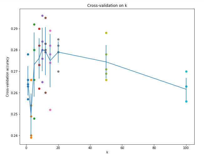
     横坐标表示不同的k值选择，纵坐标表示交叉验证的准确率。

3.19  验证k值

# Based on the cross-validation results above, choose the best value for k,   
# retrain the classifier using all the training data, and test it on the test
# data. You should be able to get above 28% accuracy on the test data.
temp = 0
for k in k_choices:
    accuracies = k_to_accuracies[k]    
    if temp < accuracies[np.argmax(accuracies)]:
        temp = accuracies[np.argmax(accuracies)]
        best_k = k
print(best_k)


classifier = KNearestNeighbor()
classifier.train(X_train, y_train)
y_test_pred = classifier.predict(X_test, k=best_k)

# Compute and display the accuracy
num_correct = np.sum(y_test_pred == y_test)
accuracy = float(num_correct) / num_test
print('Got %d / %d correct => accuracy: %f' % (num_correct, num_test, accuracy))

   我们找到最佳k值，利用测试集验证。结果如下：

10
Got 141 / 500 correct => accuracy: 0.282000

       需要指出的是，训练集、验证集和测试集是不同的三个集合。训练集是训练用的数据，在其中分裂出一部分作为验证集，用来参数调优；记住千万不能利用测试集来调优，它应该是最后用来检验模型能力的标准。

总结

        可以看到，KNN模型用作图像分类任务是没有优势的，训练很简单（保存数据），测试的时候很耗费时间和计算资源（一一比对计算）。即使是最好的情况，识别率也不足30%。我们用这个模型来熟悉图像分类的大致流程，训练我们的向量化思维。

最后

以上就是精明手机为你收集整理的CS231n Assiganment#1解析（一）——KNN前言一、准备工作二、作业解析总结的全部内容，希望文章能够帮你解决CS231n Assiganment#1解析（一）——KNN前言一、准备工作二、作业解析总结所遇到的程序开发问题。

如果觉得靠谱客网站的内容还不错，欢迎将靠谱客网站推荐给程序员好友。