这段时间在学习TensorFlow,这些都是一些官网上的例子,在这里和大家分享记录一下。
出自:https://www.tensorflow.org/tutorials/keras/basic_classification
本指南训练神经网络模型,对运动鞋和衬衫等服装图像进行分类。如果您不了解所有细节,这是可以的,这是一个完整的TensorFlow程序的快节奏概述,详细解释了我们的细节。
本指南使用tf.keras,一个高级API,用于在TensorFlow中构建和训练模型。
一、导入库
主要使用的3个库:
# TensorFlow and tf.keras
import tensorflow as tf
from tensorflow import keras

# Helper libraries
import numpy as np
import matplotlib.pyplot as plt
导入Fashion MNIST数据集
本指南使用Fashion MNIST数据集,其中包含10个类别中的70,000个灰度图像。图像显示了低分辨率(28 x 28像素)的单件服装,如下所示:
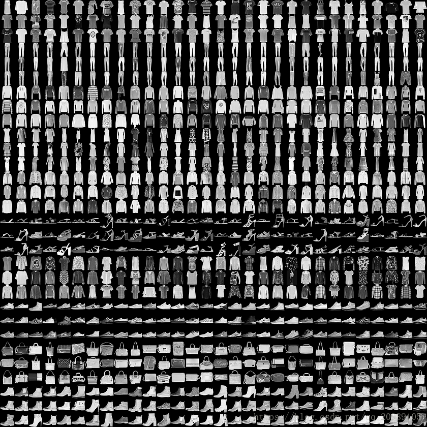
Fashion-MNIST旨在作为经典MNIST数据集的直接替代品- 通常用作计算机视觉机器学习计划的“Hello,World”。MNIST数据集包含手写数字(0,1,2等)的图像,其格式与我们在此处使用的服装相同。
本指南使用Fashion MNIST进行多样化,因为它比普通的MNIST更具挑战性。两个数据集都相对较小,用于验证算法是否按预期工作。它们是测试和调试代码的良好起点。
我们将使用60,000个图像来训练网络和10,000个图像,以评估网络学习对图像进行分类的准确程度。您可以直接从TensorFlow访问Fashion MNIST,只需导入并加载数据:
fashion_mnist = keras.datasets.fashion_mnist
(train_images, train_labels), (test_images, test_labels) = fashion_mnist.load_data()
加载数据集将返回四个NumPy数组:
- 在train_images和train_labels阵列的训练集模型使用学习-The数据。
针对测试集,数组test_images和test_labels数组测试模型。 - 图像是28x28 NumPy数组,像素值介于0到255之间。标签是一个整数数组,范围从0到9.这些对应于图像所代表的服装类别:
| 标签 | 类 |
|---|---|
| 0 | T恤衫/上衣 |
| 1 | 裤子 |
| 2 | 套衫 |
| 3 | 连衣裙 |
| 4 | 外套 |
| 5 | 凉鞋 |
| 6 | 衬衫 |
| 7 | 运动鞋 |
| 8 | 袋子 |
| 9 | 踝靴 |
每个图像都映射到一个标签。由于类名不包含在数据集中,因此将它们存储在此处以便在绘制图像时使用:
class_names = ['T-shirt/top', 'Trouser', 'Pullover', 'Dress', 'Coat',
               'Sandal', 'Shirt', 'Sneaker', 'Bag', 'Ankle boot']
探索数据
让我们在训练模型之前探索数据集的格式。以下显示训练集中有60,000个图像,每个图像表示为28 x 28像素:
train_images.shape

(60000,28,28)
同样,训练集中有60,000个标签:
len(train_labels)

60000
每个标签都是0到9之间的整数:
train_labels

数组([9,0,0,...,3,0,5],dtype = uint8)
测试集中有10,000个图像。同样,每个图像表示为28 x 28像素:
test_images.shape

(10000,28,28)
测试集包含10,000个图像标签:
len(test_labels)

10000
预处理数据
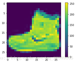
在训练网络之前,必须对数据进行预处理。如果您检查训练集中的第一个图像,您将看到像素值落在0到255的范围内:
plt.figure()
plt.imshow(train_images[0])
plt.colorbar()
plt.grid(False)
在馈送到神经网络模型之前,我们将这些值缩放到0到1的范围。为此,将图像组件的数据类型从整数转换为float,并除以255.0。
对训练集和测试集以同样的方式进行预处理,这是非常重要的:
train_images = train_images / 255.0

test_images = test_images / 255.0
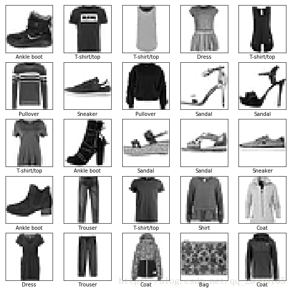
显示训练集中的前25个图像,并在每个图像下方显示类名。验证数据格式是否正确,我们是否已准备好构建和培训网络。
plt.figure(figsize=(10,10))
for i in range(25):
    plt.subplot(5,5,i+1)
    plt.xticks([])
    plt.yticks([])
    plt.grid(False)
    plt.imshow(train_images[i], cmap=plt.cm.binary)
    plt.xlabel(class_names[train_labels[i]])
建立模型
构建神经网络需要配置模型的层,然后编译模型。
设置图层
神经网络的基本构建块是层。图层从提供给它们的数据中提取表示。并且,希望这些表示对于手头的问题更有意义。
大多数深度学习包括将简单层链接在一起。大多数图层tf.keras.layers.Dense都具有在训练期间学习的参数。
model = keras.Sequential([
    keras.layers.Flatten(input_shape=(28, 28)),
    keras.layers.Dense(128, activation=tf.nn.relu),
    keras.layers.Dense(10, activation=tf.nn.softmax)
])
-
该网络中的第一层
tf.keras.layers.Flatten将图像的格式从2d阵列(28乘28像素)转换为28 * 28 = 784像素的1d阵列。可以将此图层视为图像中未堆叠的像素行并将其排列。该层没有要学习的参数; 它只重新格式化数据。 -
在像素被展平之后,网络由
tf.keras.layers.Dense两层序列组成。这些是密集连接或完全连接的神经层。第一Dense层有128个节点(或神经元)。第二(和最后)层是10节点softmax层 - 这返回10个概率分数的数组,其总和为1.每个节点包含指示当前图像属于10个类之一的概率的分数。
编译模型
在模型准备好进行培训之前,它需要更多设置。这些是在模型的编译步骤中添加的:
- 损失函数 - 这可以衡量模型在训练过程中的准确程度。我们希望最小化此功能,以便在正确的方向上“引导”模型。
- 优化器 - 这是基于它看到的数据及其损失函数更新模型的方式。
- 度量标准 - 用于监控培训和测试步骤。以下示例使用精度,即正确分类的图像的分数。
model.compile(optimizer=tf.train.AdamOptimizer(),
              loss='sparse_categorical_crossentropy',
              metrics=['accuracy'])
训练模型
训练神经网络模型需要以下步骤:
- 将训练数据提供给模型 - 在此示例中为train_images和train_labels数组。
- 该模型学会了关联图像和标签。
- 我们要求模型对测试集进行预测 - 在这个例子中,test_images数组。我们验证预测是否与test_labels数组中的标签匹配。
要开始训练,请调用model.fit方法 - 模型“适合”训练数据:
model.fit(train_images, train_labels, epochs=5)
输出:
Epoch 1/5
60000/60000 [==============================] - 6s 98us/step - loss: 0.4998 - acc: 0.8244
Epoch 2/5
60000/60000 [==============================] - 5s 90us/step - loss: 0.3767 - acc: 0.8643
Epoch 3/5
60000/60000 [==============================] - 8s 136us/step - loss: 0.3384 - acc: 0.8768
Epoch 4/5
60000/60000 [==============================] - 7s 122us/step - loss: 0.3129 - acc: 0.8852
Epoch 5/5
60000/60000 [==============================] - 5s 83us/step - loss: 0.2957 - acc: 0.8915
10000/10000 [==============================] - 0s 44us/step
Test accuracy: 0.8696
随着模型训练,显示损失和准确度指标。该模型在训练数据上达到约0.88(或88%)的准确度。
评估准确性
接下来,比较模型在测试数据集上的执行情况:
test_loss, test_acc = model.evaluate(test_images, test_labels)

print('Test accuracy:', test_acc)
输出:
Test accuracy: 0.8696
事实证明,测试数据集的准确性略低于训练数据集的准确性。训练精度和测试精度之间的差距是过度拟合的一个例子。过度拟合是指机器学习模型在新数据上的表现比在训练数据上表现更差。
作出预测
通过训练模型,我们可以使用它来预测某些图像。
predictions = model.predict(test_images)
这里,模型已经预测了测试集中每个图像的标签。我们来看看第一个预测:
predictions[0]
阵列([1.9905892e-06,1.2566167e-08,6.98845036e-08,1.0045448e-08,
       1.8485264e-07,7.5045829e-03,6.9550931e-07,4.9028788e-02,
       4.0079590e-07,9.4346321e-01],dtype = float32)
预测是10个数字的数组。这些描述了模型的“信心”,即图像对应于10种不同服装中的每一种。我们可以看到哪个标签具有最高的置信度值:
np.argmax(predictions[0])

9
因此,该模型最有信心这个图像是踝靴,或class_names[9]。我们可以检查测试标签,看看这是否正确:
test_labels[0]

9
我们可以用图表来查看全部的10个类别:
def plot_image(i, predictions_array, true_label, img):
  predictions_array, true_label, img = predictions_array[i], true_label[i], img[i]
  plt.grid(False)
  plt.xticks([])
  plt.yticks([])

  plt.imshow(img, cmap=plt.cm.binary)

  predicted_label = np.argmax(predictions_array)
  if predicted_label == true_label:
    color = 'blue'
  else:
    color = 'red'

  plt.xlabel("{} {:2.0f}% ({})".format(class_names[predicted_label],
                                100*np.max(predictions_array),
                                class_names[true_label]),
                                color=color)

def plot_value_array(i, predictions_array, true_label):
  predictions_array, true_label = predictions_array[i], true_label[i]
  plt.grid(False)
  plt.xticks([])
  plt.yticks([])
  thisplot = plt.bar(range(10), predictions_array, color="#777777")
  plt.ylim([0, 1])
  predicted_label = np.argmax(predictions_array)

  thisplot[predicted_label].set_color('red')
  thisplot[true_label].set_color('blue')
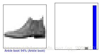
看看测试数据的第0个图像,预测和预测数组。
i = 0
plt.figure(figsize=(6,3))
plt.subplot(1,2,1)
plot_image(i, predictions, test_labels, test_images)
plt.subplot(1,2,2)
plot_value_array(i, predictions,  test_labels)
i = 12
plt.figure(figsize=(6,3))
plt.subplot(1,2,1)
plot_image(i, predictions, test_labels, test_images)
plt.subplot(1,2,2)
plot_value_array(i, predictions,  test_labels)
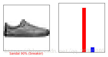
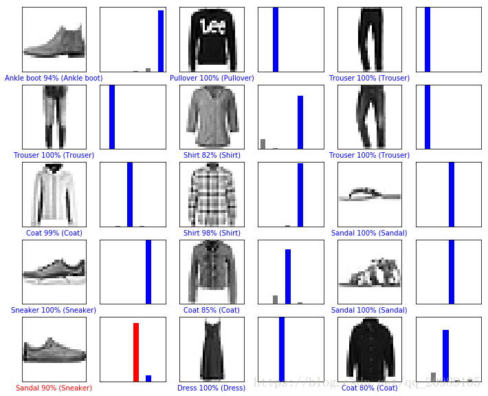
让我们用它的预测绘制几个图像。正确的预测标签是蓝色的,不正确的预测标签是红色的。该数字给出了预测标签的百分比(满分100)。请注意,即使非常自信,也可能出错。
# Plot the first X test images, their predicted label, and the true label
# Color correct predictions in blue, incorrect predictions in red
num_rows = 5
num_cols = 3
num_images = num_rows*num_cols
plt.figure(figsize=(2*2*num_cols, 2*num_rows))
for i in range(num_images):
  plt.subplot(num_rows, 2*num_cols, 2*i+1)
  plot_image(i, predictions, test_labels, test_images)
  plt.subplot(num_rows, 2*num_cols, 2*i+2)
  plot_value_array(i, predictions, test_labels)
最后,使用训练的模型对单个图像进行预测。
img = test_images[0]
print(img.shape)

#(28,28)
tf.keras模型优化,使在预测批一次,或收集的一个例子。因此,即使我们使用单个图像,我们也需要将其添加到列表中:
img = (np.expand_dims(img,0))
print(img.shape)
#(1,28,28)
现在预测图像:
predictions_single = model.predict(img)
print(predictions_single)
输出:
[[1.9905854e-06 1.2566143e-08 6.9844901e-08 1.0045391e-08 1.8485194e-07
      7.5045791e-03 6.9566664e-07 4.9028799e-02 4.0079516e-07 9.4346321e-01]]
图像:
    plot_value_array(0, predictions_single, test_labels)
    _ = plt.xticks(range(10), class_names, rotation=45)
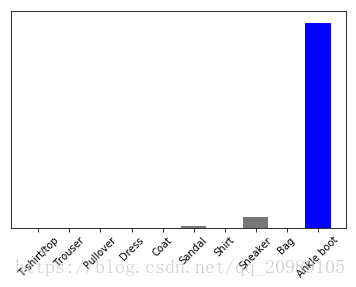
model.predict返回列表列表,每个列表对应一批数据中的每个图像。抓取批次中我们(仅)图像的预测:
np.argmax(predictions_single[0])
# 9
而且,和以前一样,模型预测标签为9。
附上完整代码:
# -*- coding: utf-8 -*-
"""
Created on Tue Sep 18 09:42:55 2018

@author: chenyang
"""

# TensorFlow and tf.keras
import tensorflow as tf
from tensorflow import keras

# Helper libraries
import numpy as np
import matplotlib.pyplot as plt

print(tf.__version__)

#绘制测试数据的图片
def plot_image(i, predictions_array, true_label, img):
  predictions_array, true_label, img = predictions_array[i], true_label[i], img[i]
  plt.grid(False)
  plt.xticks([])
  plt.yticks([])

  plt.imshow(img, cmap=plt.cm.binary)

  predicted_label = np.argmax(predictions_array)
  if predicted_label == true_label:
    color = 'blue'
  else:
    color = 'red'

  plt.xlabel("{} {:2.0f}% ({})".format(class_names[predicted_label],
                                100*np.max(predictions_array),
                                class_names[true_label]),
                                color=color)
#绘制分类结果:正确的预测标签是蓝色的,不正确的预测标签是红色的
def plot_value_array(i, predictions_array, true_label):
  predictions_array, true_label = predictions_array[i], true_label[i]
  plt.grid(False)
  plt.xticks([])
  plt.yticks([])
  thisplot = plt.bar(range(10), predictions_array, color="#777777")
  plt.ylim([0, 1])
  predicted_label = np.argmax(predictions_array)

  thisplot[predicted_label].set_color('red')
  thisplot[true_label].set_color('blue')

if __name__ == '__main__':
    fashion_mnist = keras.datasets.fashion_mnist

    #加载数据
    (train_images, train_labels), (test_images, test_labels) = fashion_mnist.load_data()

    #每个分类对应名称
    class_names = ['T-shirt/top', 'Trouser', 'Pullover', 'Dress', 'Coat',
                   'Sandal', 'Shirt', 'Sneaker', 'Bag', 'Ankle boot']

    #特征缩放
    train_images = train_images / 255.0
    test_images = test_images / 255.0

    #print(np.shape(train_images[1]))
    #显示训练集的钱25个图像
    #plt.figure()
    #plt.imshow(train_images[0])
    #plt.colorbar()
    #plt.grid(False)
    plt.figure(figsize=(10,10))
    for i in range(16):
        plt.subplot(4,4,i+1)
        plt.xticks([])
        plt.yticks([])
        plt.grid(False)
        plt.imshow(train_images[i], cmap=plt.cm.binary)
        plt.xlabel(class_names[train_labels[i]])

    #设置图层
    #第一层tf.keras.layers.Flatten将图像的格式从2d阵列(28乘28像素)转换为28 * 28 = 784像素的1d阵列
    #第一Dense层有128个节点(或神经元)。
    #第二(和最后)层是10节点softmax层 - 这返回10个概率分数的数组,其总和为1.
    #每个节点包含指示当前图像属于10个类之一的概率的分数。
    model = keras.Sequential([
        keras.layers.Flatten(input_shape=(28, 28)),
        keras.layers.Dense(128, activation=tf.nn.relu),
        keras.layers.Dense(10, activation=tf.nn.softmax)
    ])

    #参数设置
    #损失函数 - 这可以衡量模型在训练过程中的准确程度。我们希望最小化此功能,以便在正确的方向上“引导”模型。
    #优化器 - 这是基于它看到的数据及其损失函数更新模型的方式。
    #度量标准 - 用于监控培训和测试步骤。以下示例使用精度,即正确分类的图像的分数
    model.compile(optimizer=tf.train.AdamOptimizer(),
                  loss='sparse_categorical_crossentropy',
                  metrics=['accuracy'])

    #训练数据
    model.fit(train_images, train_labels, epochs=5)

    #评估准确性
    test_loss, test_acc = model.evaluate(test_images, test_labels)
    print('Test accuracy:', test_acc)

    #预测,结果为一个10个数字的数组
#    predictions = model.predict(test_images)

    #获取10个分类中的分数最高的一个
#    np.argmax(predictions[0])

#    绘制图像
#    num_rows = 5
#    num_cols = 3
#    num_images = num_rows*num_cols
#    plt.figure(figsize=(2*2*num_cols, 2*num_rows))
#    for i in range(num_images):
#        plt.subplot(num_rows, 2*num_cols, 2*i+1)
#        plot_image(i, predictions, test_labels, test_images)
#        plt.subplot(num_rows, 2*num_cols, 2*i+2)
#        plot_value_array(i, predictions, test_labels)

#    预测一个数据
    img = test_images[0]
    print(img.shape)

    img = (np.expand_dims(img,0))
    print(img.shape)

    predictions_single = model.predict(img)
    print(predictions_single)

    plot_value_array(0, predictions_single, test_labels)
#    _ = plt.xticks(range(10), class_names, rotation=45)

    print(np.argmax(predictions_single[0]))
最后
以上就是大方墨镜最近收集整理的关于TensorFlow之tf.keras的基础分类的全部内容,更多相关TensorFlow之tf.keras内容请搜索靠谱客的其他文章。


发表评论 取消回复