文章目录
- 数据分析 第七讲 pandas练习 数据的合并和分组聚合
- 一、pandas-DataFrame
- 练习1
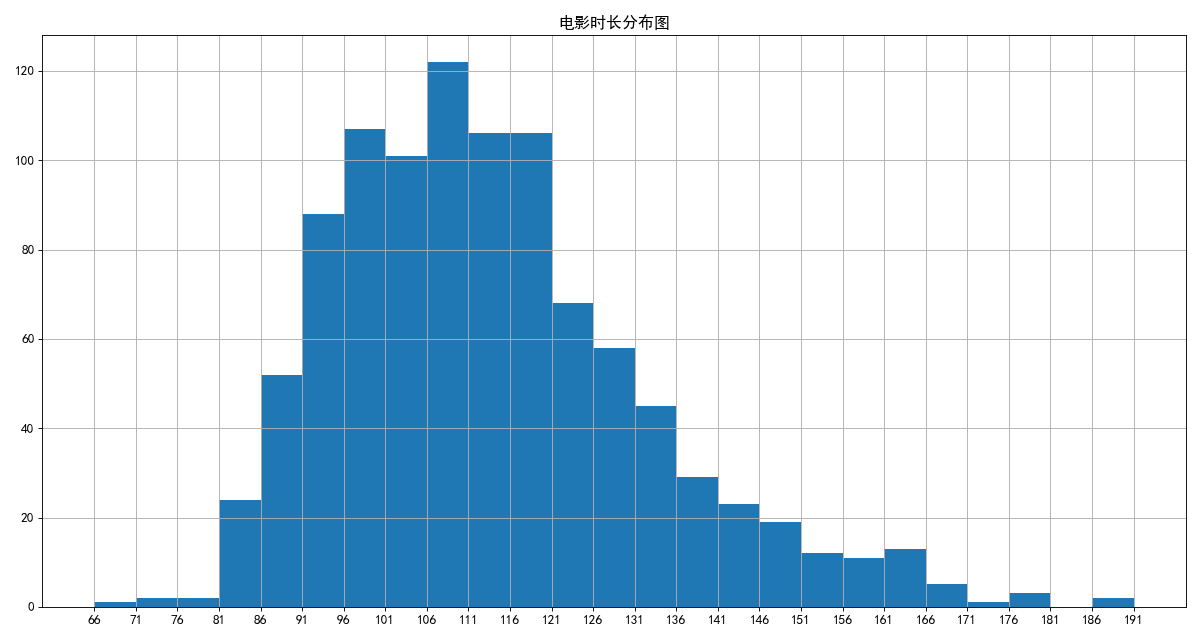
- 对于这一组电影数据,如果我们想runtime(电影时长)的分布情况,应该如何呈现数据?
- 练习2
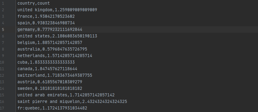
- 全球食品数据分析
- 二、数据的合并和分组聚合
- 1.字符串离散化
- 2.数据合并
- 3.数据的分组聚合
- 4.索引和复合索引
- Series复合索引
- DateFrame复合索引
- 5.练习
- 1.使用matplotlib呈现出店铺总数排名前10的国家
- 2.使用matplotlib呈现出中国每个城市的店铺数量
- 三、pandas中的时间序列
- 1.时间范围
- 2.DataFrame中使用时间序列
- 3.pandas重采样
- 4.练习
- 练习1:统计出911数据中不同月份的电话次数
- 练习2现在我们有北上广、深圳、和沈阳5个城市空气质量数据,请绘制出5个城市的PM2.5随时间的变化情况
- 四、pandas画图
- 1.折线图
- 2.分组柱状图
- 2.饼图
数据分析 第七讲 pandas练习 数据的合并和分组聚合

一、pandas-DataFrame
练习1
对于这一组电影数据,如果我们想runtime(电影时长)的分布情况,应该如何呈现数据?
数据分析
# 对于这一组电影数据,如果我们想runtime(电影时长)的分布情况,应该如何呈现数据?

import pandas as pd
from matplotlib import pyplot as plt
import matplotlib
font = {
'family':'SimHei',
'weight':'bold',
'size':12
}
matplotlib.rc("font", **font)
file_path = './IMDB-Movie-Data.csv'
df = pd.read_csv(file_path)
# print(df.info())
'''
<class 'pandas.core.frame.DataFrame'>
RangeIndex: 1000 entries, 0 to 999
Data columns (total 12 columns):
 #   Column              Non-Null Count  Dtype
---  ------              --------------  -----
 0   Rank                1000 non-null   int64
 1   Title               1000 non-null   object
 2   Genre               1000 non-null   object
 3   Description         1000 non-null   object
 4   Director            1000 non-null   object
 5   Actors              1000 non-null   object
 6   Year                1000 non-null   int64
 7   Runtime (Minutes)   1000 non-null   int64
 8   Rating              1000 non-null   float64
 9   Votes               1000 non-null   int64
 10  Revenue (Millions)  872 non-null    float64
 11  Metascore           936 non-null    float64
dtypes: float64(3), int64(4), object(5)
memory usage: 93.9+ KB
None
'''
# print(df.head(3))
# runtime_data = df.loc[:,'Runtime (Minutes)']  # 也可以直接取runtime_data = df['Runtime (Minutes)']
# print(type(runtime_data))  # <class 'pandas.core.series.Series'>
runtime_data = df['Runtime (Minutes)']
print(type(runtime_data))  # <class 'pandas.core.series.Series'>
print(max(runtime_data))  # 191
print(min(runtime_data))  # 66
# print(runtime_data)
'''
0      121
1      124
2      117
3      108
4      123
      ...
995    111
996     94
997     98
998     93
999     87
Name: Runtime (Minutes), Length: 1000, dtype: int64
'''
runtime_data = df['Runtime (Minutes)'].values  # 变成列表的形式
print(type(runtime_data))  # <class 'numpy.ndarray'>
print(max(runtime_data))  # 191
print(min(runtime_data))  # 66
# print(runtime_data)
'''
[121 124 117 108 123 103 128  89 141 116 133 127 133 107 109  87 139 123
 118 116 120 137 108  92 120  83 159  99 100 115 111 116 144 108 107 147
 169 115 132 113  89 111  73 115  99 136 132  91 122 130 136  91 118 101
 152 161  88 106 117  96 151  86 112 125 130 129 133 120 106 107 133 124
 108  97 108 169 143 153 151 116 148 118 180 149 137 124 129 162 187 128
 153 123 146 114 141 116 106  90 105 151 132 115 144 106 116 102 120 110
 105 108  89 134 118 117 130 105 118 161 104  97 127 139  98  86 164 106
 165  96 108 156 139 125  86 107 130 140 122 143 138 148 127  94 130 118
 165 144 104 162 113 121 117 142  88 121  91  94 131 118 112 121 106  90
 132 118 144 122 129 109 144 148 118 101  84 126 102 130 130 107 134 117
 118  92 105 112 124 135 113 119 100 125 133  94 128  92 140 124  95 148
 114 107 113 146 134 126 120 132  99 118 125 111 114  94 144 104 112 126
 136 104 100 117  96 117 100 158 110 163 119 107  97 102 118  95 139 131
 114 102 100  85  99 125 134  95  90 126 118 158 109 119 119 112  92  94
 147 142 112 100 131 105  81 118 119 108 108 117 112  99 102 172 107  85
 143 169 110 106  89 124 112 157 117 130 115 128 113 119  98 110 105 127
  95  99 118 112  92 107 143 111  94 109 127 158 132 121  95  97 104 148
 113 110 104 110 129 180  93 144 138 126 112  81  94 131 104  84 114 109
 120 106 110 103  95 133  87 133 117 150 123  97 122  88 126 117 107 119
 131 102 139 110 127 138 102  94  89 124 119  96 119 102 118 123 107 123
  98 100 132  88 106 120 115 117 136 123  89 113 113 110 111  99 123 133
  97 126  86 124  81 142 100 121 105 140 126 132 100 115 122  98 101 112
 112 113  85 110  91  91  92  95 118 100 157 100 137  99  93 115 104 130
  98 102 108 123 146 101 111  88 108 102  99 166 102 115 104 109 170 102
 116 132 102  97 123 114 103  88 130 117 100 112  81 125  95 101 102 100
 124 101 108 119 109 115 108 100 117 119 125  97 109  97 103 129 100  91
 112 107 157 123 158 153 120 106 137  94  96 113 111  97 115  97  97  94
 117 115 105 111  98 118  85 114 108 101 106 112 109  96 131 118 109 124
 141 110 131  95  94  91  94 124  91 132 115  92 150 120 161 111 120 117
 133 112 106 103 109 100 123 135 117  92 126  89 125 132 130 108  92 108
 128 105 107 126 103 112  92 108  98 100 106 123 100 104 106  91 108  92
 122  84 103  91 110 101 127 111 154  96  98  98 109 107 121 101 117 106
 117 125 146 101  90 103  94 110 133 114 137 110 107  93 152 112 106 105
  96 116 110  83  97  95 113  88 129  95 110  95 100  98 139 120 124 162
 135 160  90  92 101 139  95 114 103  88 108  97 109 118 104  88  93  98
 112 112 120  85  98 129  93 116  83 113 117 122 119 113  85 116 101 133
 101 104 116 101 103  87  83 140 165 101 100  96 111  95 114 117 102 129
 106 115 129 143 114 137 131 114  98 126 115 102 101 140 123 112  90 130
 123 118  96  88 103 122  96 151 104 105 127  93 100 106 128  94 111 106
 111 165  98  87 106  88 141  96 150  80  95 131 116 108 104  86 138  97
 123 115 102  89 140 113 109 110 117 100 119 104 100 149 104 126  93 128
 118 112  99 111 129 110  96 116  86 127  99 106 113 104 107 103 106 111
  92  87 113 116 114 114 102 118  85 153 114 122 109 119 106  95  98 110
  96 106 102  90  90 108 113 117 120  82  95 134 108  92  89  92 118 111
 101  66 102 108 120  98 114 109  88 110 115 105 104 111 116  95 111 128
  93 100 123 112  87 129  95  94  99  73 107 123 118 119  90  88  91 108
 191  87 102  94 120 112  83 108 128 113 102 115 108 125 135  97  98 138
  94 131 108 128 123 104 116  96  92 111 115 123 107 141 113 129  81  85
 108 120 110 122  99 126 116  85  93 107 114 100  98  98 110  99 120 125
 119  96 101 143 139 101  88 100 104 134 127 145  92 105 123 117  96  89
 101 105  98 102 117 110  95 122  95 106 133  87  96  89 122 156 103  91
 147 113  97  93 102 103 154 117 110 110  86 144 113 107  97  97 120 108
  92  96 108 109  98 124  86 106 119  99 132  91 100  80 105 115 146  95
 105  94 100 109 117 110 101 101 115 108 104 180 122 123  83 150  92 105
 123 111 124  94 113  92  97 120 109 118 133 104 111 102  92 104  99 128
  92 165  97  97  88 111  94  98  93  87]'''
max_runtime = max(runtime_data)
min_runtime = min(runtime_data)

# 直方图
# 组数 = (最大值-最小值)/组距  (191-66)//5 = 25
num_bins = (max_runtime - min_runtime) // 5
# print(num_bins)  # 25

plt.figure(figsize=(15,8),dpi=80)
plt.hist(runtime_data,num_bins)
plt.xticks(range(min_runtime,max_runtime+5,5))
plt.title('电影时长分布图')
plt.grid()
plt.show()
练习2
全球食品数据分析
步骤分析
1.数据清洗
2.获取国家列表
3.对各个国家进行统计
4.保存统计结果
import pandas as pd

# df = pd.read_csv('FoodFacts.csv')
# print(df.info())
'''
sys:1: DtypeWarning: Columns (0,3,5,27,36) have mixed types.Specify dtype option on import or set low_memory=False.
<class 'pandas.core.frame.DataFrame'>
RangeIndex: 65503 entries, 0 to 65502
Columns: 159 entries, code to nutrition_score_uk_100g
dtypes: float64(103), object(56)
memory usage: 79.5+ MB
None'''


def get_countries(countries_data):
    '''获取国家数据'''
    low_countries_data = countries_data.str.lower()  # 改为小写
    # print(low_countries_data.head(30))
    # 很多行包含两个国家france,united kingdom
    # contains 模糊查询  ~ 非
    low_countries_data = low_countries_data[~low_countries_data.str.contains(',')]
    countries = low_countries_data.unique()  # 返回列的所有唯一值
    # print(countries)
    '''
    ['united kingdom' 'france' 'spain' 'germany' 'united states' 'belgium'
     'australia' 'netherlands' 'cuba' 'canada' 'switzerland' 'austria'
     'sweden' 'united arab emirates' 'saint pierre and miquelon' 'fr:quebec'
     'italy' 'czech republic' 'china' 'cambodia' 'réunion' 'hong kong'
     'brazil' 'japan' 'mexico' 'lebanon' 'philippines' 'guadeloupe' 'ireland'
     'senegal' "côte d'ivoire" 'togo' 'poland' 'india' 'south korea' 'turkey'
     'french guiana' 'portugal' 'south africa' 'romania' 'denmark' 'greece'
     'luxembourg' 'new caledonia' 'russia' 'french polynesia' 'tunisia'
     'martinique' 'mayotte' 'hungary' 'bulgaria' 'slovenia' 'finland'
     'republique-de-chine' 'taiwan' 'lithuania' 'belarus' 'cyprus' 'irlande'
     'albania' 'malta' 'iceland' 'polska' 'kenya' 'mauritius' 'algeria' 'iran'
     'qatar' 'thailand' 'colombia' 'norway' 'israel' 'venezuela' 'argentina'
     'chile' 'new zealand' 'andorra' 'serbia' 'other-turquie' 'iraq'
     'nederland' 'singapore' 'indonesia' 'burkina faso']'''
    # print("一共有%s个国家"%len(countries))  # 一共有84个国家
    return countries


def get_additives_count(countries, data):
    count_list = []
    for country in countries:
        f_data = data[data['countries_en'].str.contains(country, case=False)]  # 模糊查找,不区分大小写
        # print(f_data.head(10))
        # exit()
        '''
                             countries_en  additives_n
        5          United Kingdom          0.0
        10         United Kingdom          5.0
        11         United Kingdom          5.0
        14         United Kingdom          0.0
        17         United Kingdom          0.0
        18         United Kingdom          0.0
        46  France,United Kingdom          1.0
        60         United Kingdom          0.0
        84         United Kingdom          0.0
        97         United Kingdom          0.0
        '''
        count = f_data['additives_n'].mean()  # 计算平均值
        count_list.append(count)
    # print(count_list)
    '''
    [1.259009009009009, 1.93042170523602, 0.930323846908734, 0.7779232111692844, 2.1806083650190113, 1.8857142857142857, 0.5796847635726795, 1.5714285714285714, 1.8333333333333333, 1.847457627118644, 1.7183673469387755, 0.6185567010309279, 0.18181818181818182, 1.7142857142857142, 2.4324324324324325, 1.1724137931034482, 0.9190751445086706, 1.2666666666666666, 1.2, 0.2222222222222222, 2.0625, 1.375, 0.898876404494382, 0.8666666666666667, 1.75, 0.6, 0.8, 1.6748466257668713, 0.7142857142857143, 1.9166666666666667, 0.0, 8.0, 2.310810810810811, 2.0, 2.0, 0.3, 1.7954545454545454, 1.8299492385786802, 1.7272727272727273, 1.7692307692307692, 1.5912408759124088, 1.1111111111111112, 2.1923076923076925, 1.3333333333333333, 0.125, 2.0, 2.246153846153846, 1.5454545454545454, 0.0, 0.5384615384615384, 1.25, 0.25, 0.4166666666666667, 1.0, 0.0, 1.0, 0.0, 0.0, 0.0, 0.2857142857142857, 1.3333333333333333, 0.6666666666666666, 0.0, 1.5, 2.1666666666666665, 2.857142857142857, 0.0, 4.4, 0.6896551724137931, 0.5, 1.5714285714285714, 1.0, 0.0, 1.9090909090909092, 3.5, 2.6607142857142856, 0.2, 2.0, 0.0, 1.5, 0.0, 1.0, 2.125, 1.6666666666666667]
    '''
    # print(len(count_list))  # 84
    result_df = pd.DataFrame()
    result_df['country'] = countries
    result_df['count'] = count_list
    return result_df


def main():
    '''主函数'''
    # 读取数据
    df1 = pd.read_csv('FoodFacts.csv', usecols=['countries_en', 'additives_n'])
    # print(df1.info())
    '''
    <class 'pandas.core.frame.DataFrame'>
    RangeIndex: 65503 entries, 0 to 65502
    Data columns (total 2 columns):
     #   Column        Non-Null Count  Dtype
    ---  ------        --------------  -----
     0   countries_en  65292 non-null  object
     1   additives_n   43664 non-null  float64
    dtypes: float64(1), object(1)
    memory usage: 1023.6+ KB
    None'''
    # 数据清洗  删除缺失数据
    data = df1.dropna()
    # print(data.info())
    '''<class 'pandas.core.frame.DataFrame'>
    Int64Index: 43616 entries, 5 to 65501
    Data columns (total 2 columns):
     #   Column        Non-Null Count  Dtype
    ---  ------        --------------  -----
     0   countries_en  43616 non-null  object
     1   additives_n   43616 non-null  float64
    dtypes: float64(1), object(1)
    memory usage: 1022.2+ KB
    None'''
    # print(data.head())
    '''      countries_en  additives_n
    5   United Kingdom          0.0
    6           France          0.0
    8           France          0.0
    10  United Kingdom          5.0
    11  United Kingdom          5.0'''

    countries = get_countries(data['countries_en'])
    # print(countries)
    # 获取每个国家添加剂的数量
    additives = get_additives_count(countries, data)
    additives.to_csv('result.csv', index=False)  # 保存,不加索引


if __name__ == "__main__":
    main()
二、数据的合并和分组聚合
1.字符串离散化
- 字符串离散化的案例
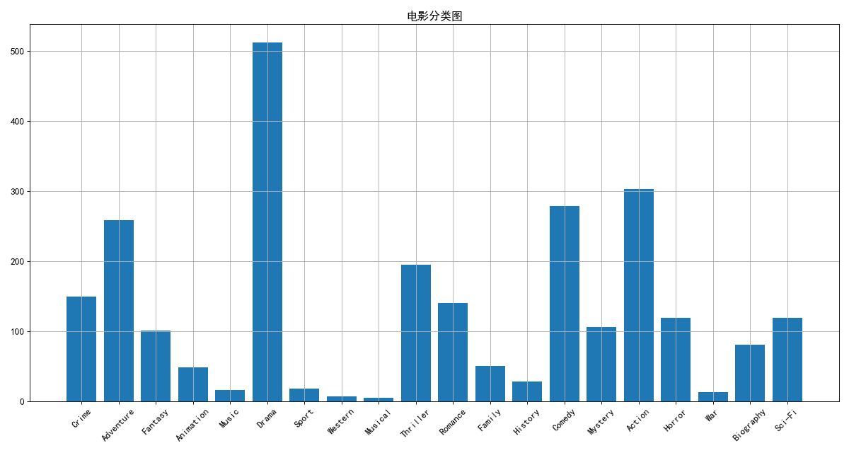
对于这一组电影数据,如果我们希望统计电影分类(genre)的情况,应该如何处理数据? - 思路:重新构造一个全为0的数组,列名为分类,如果某一条数据中分类出现过,就让0变为1

# 字符串离散化的案例
import pandas as pd
import numpy as np
from matplotlib import pyplot as plt
import matplotlib

font = {
    'family': 'SimHei',
    'weight': 'bold',
    'size': 12
}
matplotlib.rc("font", **font)

pd.set_option('display.max_columns', None)
pd.set_option('display.max_rows', 5)  # 只看5行
pd.set_option('max_colwidth', 200)

file_path = './IMDB-Movie-Data.csv'

df = pd.read_csv(file_path)
# print(df)
# print(df.info())
# print(df.head(3))
g_list = df.loc[:, 'Genre']  # 获取分类列
# print(g_list)
'''
0       Action,Adventure,Sci-Fi
1      Adventure,Mystery,Sci-Fi
                 ...
998            Adventure,Comedy
999       Comedy,Family,Fantasy
Name: Genre, Length: 1000, dtype: object'''
g_list = df["Genre"].str.split(",").tolist()  # [[],...,[]]
# print(g_list)
# temp_list = []
# for i in g_list:
#     for j in i:
#         # print(j)
#         temp_list.append(j)
# print(set(temp_list))
genre_list = list(set([j for i in g_list for j in i]))  # 电影分类类名
# print(genre_list)
'''['Action', 'Crime', 'Biography', 'Adventure', 'Thriller', 'Music', 'Romance', 'Sport', 'Family', 'Horror', 'Western', 'War', 'Animation', 'Mystery', 'Sci-Fi', 'History', 'Drama', 'Musical', 'Fantasy', 'Comedy']'''

# 构造全为0的数组
zeros_data = pd.DataFrame(np.zeros((df.shape[0], len(genre_list))), columns=genre_list)
# print(zeros_data)
'''
     Action  Horror  Family  Thriller  Animation  History  Romance  Fantasy
0       0.0     0.0     0.0       0.0        0.0      0.0      0.0      0.0
1       0.0     0.0     0.0       0.0        0.0      0.0      0.0      0.0
..      ...     ...     ...       ...        ...      ...      ...      ...
998     0.0     0.0     0.0       0.0        0.0      0.0      0.0      0.0
999     0.0     0.0     0.0       0.0        0.0      0.0      0.0      0.0

     Biography  Western  Drama  Comedy  Sci-Fi  Crime  War  Sport  Mystery
0          0.0      0.0    0.0     0.0     0.0    0.0  0.0    0.0      0.0
1          0.0      0.0    0.0     0.0     0.0    0.0  0.0    0.0      0.0
..         ...      ...    ...     ...     ...    ...  ...    ...      ...
998        0.0      0.0    0.0     0.0     0.0    0.0  0.0    0.0      0.0
999        0.0      0.0    0.0     0.0     0.0    0.0  0.0    0.0      0.0

     Musical  Music  Adventure
0        0.0    0.0        0.0
1        0.0    0.0        0.0
..       ...    ...        ...
998      0.0    0.0        0.0
999      0.0    0.0        0.0

[1000 rows x 20 columns]'''

# 给每个电影出现的位置赋值1
# print(df)  # [1000 rows x 12 columns]
for i in range(df.shape[0]):
    # zeros_data[0,[Action,Musical]] = 1
    zeros_data.loc[i, g_list[i]] = 1
# print(zeros_data.head(3))
'''
   Music  Sport  Mystery  Adventure  Musical  Comedy  Horror  Fantasy  Action
0    0.0    0.0      0.0        1.0      0.0     0.0     0.0      0.0     1.0
1    0.0    0.0      1.0        1.0      0.0     0.0     0.0      0.0     0.0
2    0.0    0.0      0.0        0.0      0.0     0.0     1.0      0.0     0.0

   Biography  Family  Sci-Fi  War  Thriller  Romance  Drama  Crime  Animation
0        0.0     0.0     1.0  0.0       0.0      0.0    0.0    0.0        0.0
1        0.0     0.0     1.0  0.0       0.0      0.0    0.0    0.0        0.0
2        0.0     0.0     0.0  0.0       1.0      0.0    0.0    0.0        0.0

   Western  History
0      0.0      0.0
1      0.0      0.0
2      0.0      0.0
'''
genre_count = zeros_data.sum(axis=0)  # 对0轴进行求和
# print(genre_count)
'''
Thriller     195.0
Biography     81.0
             ...
Action       303.0
Sci-Fi       120.0
Length: 20, dtype: float64'''

x = genre_count.index
y = genre_count.values

plt.figure(figsize=(15, 8), dpi=80)
plt.bar(x, y)
plt.xticks(range(len(x)), x, rotation=45)
plt.title("电影分类图")
plt.grid()
plt.show()
2.数据合并
- join:默认情况下它是把行索引相同的数据合并到一起
- merge:按照指定的列把数据按照一定的方式合并到一起
- 示例1
# 数据合并
import numpy as np
import pandas as pd

t1 = pd.DataFrame(np.arange(12).reshape(3,4),index=list('ABC'),columns=list('DEFG'))
t2 = pd.DataFrame(np.arange(10).reshape(2,5),index=list('AB'),columns=list('VWXYZ'))
print(t1)
'''
   D  E   F   G
A  0  1   2   3
B  4  5   6   7
C  8  9  10  11'''
print(t2)
'''
   V  W  X  Y  Z
A  0  1  2  3  4
B  5  6  7  8  9'''
print(t1 + t2)
'''
    D   E   F   G   V   W   X   Y   Z
A NaN NaN NaN NaN NaN NaN NaN NaN NaN
B NaN NaN NaN NaN NaN NaN NaN NaN NaN
C NaN NaN NaN NaN NaN NaN NaN NaN NaN'''

print(t1.join(t2))  # join:以t1为基础,默认情况下它是把行索引相同的数据合并到一起
'''
   D  E   F   G    V    W    X    Y    Z
A  0  1   2   3  0.0  1.0  2.0  3.0  4.0
B  4  5   6   7  5.0  6.0  7.0  8.0  9.0
C  8  9  10  11  NaN  NaN  NaN  NaN  NaN'''
print(t2.join(t1))  # join:以t2为基础,默认情况下它是把行索引相同的数据合并到一起
'''
   V  W  X  Y  Z  D  E  F  G
A  0  1  2  3  4  0  1  2  3
B  5  6  7  8  9  4  5  6  7'''
t3 = pd.DataFrame(np.arange(12).reshape(3,4),index=list('ABC'),columns=list('DEFG'))
t4 = pd.DataFrame(np.arange(10).reshape(2,5),index=list('AC'),columns=list('VWXYZ'))
print(t3)
'''
   D  E   F   G
A  0  1   2   3
B  4  5   6   7
C  8  9  10  11'''
print(t4)
'''
   V  W  X  Y  Z
A  0  1  2  3  4
C  5  6  7  8  9'''
print(t3.join(t4))  # join:以t3为基础,默认情况下它是把行索引相同的数据合并到一起
'''
   D  E   F   G    V    W    X    Y    Z
A  0  1   2   3  0.0  1.0  2.0  3.0  4.0
B  4  5   6   7  NaN  NaN  NaN  NaN  NaN
C  8  9  10  11  5.0  6.0  7.0  8.0  9.0'''
print(t4.join(t3))  # join:以t4为基础,默认情况下它是把行索引相同的数据合并到一起
'''
   V  W  X  Y  Z  D  E   F   G
A  0  1  2  3  4  0  1   2   3
C  5  6  7  8  9  8  9  10  11'''
t5 = pd.DataFrame(np.arange(12).reshape(3,4),index=list('ABC'),columns=list('DEFG'))
t6 = pd.DataFrame(np.arange(10).reshape(2,5),index=list('DE'),columns=list('VWXYZ'))
print(t5.join(t6))  # join:以t5为基础,没有相同的索引,后面拼接的都为NaN
'''
   D  E   F   G   V   W   X   Y   Z
A  0  1   2   3 NaN NaN NaN NaN NaN
B  4  5   6   7 NaN NaN NaN NaN NaN
C  8  9  10  11 NaN NaN NaN NaN NaN'''
print(t6.join(t5))  # join:以t6为基础,没有相同的索引,后面拼接的都为NaN
'''
   V  W  X  Y  Z   D   E   F   G
D  0  1  2  3  4 NaN NaN NaN NaN
E  5  6  7  8  9 NaN NaN NaN NaN'''
- 示例2
# 数据合并
import numpy as np
import pandas as pd

t1 = pd.DataFrame(np.arange(12).reshape(3, 4), index=list('ABC'), columns=list('DEFG'))
t2 = pd.DataFrame(np.arange(10).reshape(2, 5), index=list('AB'), columns=list('DWXYZ'))
print(t1)
'''
   D  E   F   G
A  0  1   2   3
B  4  5   6   7
C  8  9  10  11'''
print(t2)
'''
   D  W  X  Y  Z
A  0  1  2  3  4
B  5  6  7  8  9'''
print(t1 + t2)
'''
     D   E   F   G   W   X   Y   Z
A  0.0 NaN NaN NaN NaN NaN NaN NaN
B  9.0 NaN NaN NaN NaN NaN NaN NaN
C  NaN NaN NaN NaN NaN NaN NaN NaN'''
print(t1.merge(t2))  # merge:至少要有一个相同的列索引,相同的列下有相同的元素,就把该元素所在的行(去除相同的元素)合并到一行
'''
   D  E  F  G  W  X  Y  Z
0  0  1  2  3  1  2  3  4'''
t1.iloc[2, 0] = 5
print(t1)
'''
   D  E   F   G
A  0  1   2   3
B  4  5   6   7
C  5  9  10  11'''
print(t2)
'''
   D  W  X  Y  Z
A  0  1  2  3  4
B  5  6  7  8  9'''
print(t1.merge(t2))  # 以t1为主,merge:至少要有一个相同的列索引,相同的列下有相同的元素,就把该元素所在的行(去除相同的元素)合并到一行,合并后的数据行索引从0开始
'''
   D  E   F   G  W  X  Y  Z
0  0  1   2   3  1  2  3  4
1  5  9  10  11  6  7  8  9'''
print(t2.merge(t1))  # 以t2为主,merge:至少要有一个相同的列索引,相同的列下有相同的元素,就把该元素所在的行(去除相同的元素)合并到一行,合并后的数据行索引从0开始
'''
   D  W  X  Y  Z  E   F   G
0  0  1  2  3  4  1   2   3
1  5  6  7  8  9  9  10  11'''
t1.iloc[[0, 1, 2], 0] = 1
print(t1)
'''
   D  E   F   G
A  1  1   2   3
B  1  5   6   7
C  1  9  10  11'''
print(t2)
'''
   D  W  X  Y  Z
A  0  1  2  3  4
B  5  6  7  8  9'''
print(t2.merge(t1))  # 以t2为主,merge:至少要有一个相同的列索引,相同的列下没有相同的元素,Empty DataFrame
'''
Empty DataFrame
Columns: [D, W, X, Y, Z, E, F, G]
Index: []'''
t1.iloc[[0, 1, 2], 0] = 0
print(t1)
'''
   D  E   F   G
A  0  1   2   3
B  0  5   6   7
C  0  9  10  11'''
print(t2)
'''
   D  W  X  Y  Z
A  0  1  2  3  4
B  5  6  7  8  9'''
print(t2.merge(t1))  # 以t2为主,merge:至少要有一个相同的列索引,相同的列下有相同的元素,就把该元素所在的行(去除相同的元素)合并到一行,合并后的数据行索引从0开始
'''
   D  W  X  Y  Z  E   F   G
0  0  1  2  3  4  1   2   3
1  0  1  2  3  4  5   6   7
2  0  1  2  3  4  9  10  11'''
print(t2.merge(t1,
               how='left'))  # 以t2为主,merge:至少要有一个相同的列索引,相同的列下有相同的元素,就把该元素所在的行(去除相同的元素)合并到一行,合并后的数据行索引从0开始 how='left'保留t2的原数据,后面用NaN填充
'''
   D  W  X  Y  Z    E     F     G
0  0  1  2  3  4  1.0   2.0   3.0
1  0  1  2  3  4  5.0   6.0   7.0
2  0  1  2  3  4  9.0  10.0  11.0
3  5  6  7  8  9  NaN   NaN   NaN'''
print(t2.merge(t1, on='D', how='outer'))
'''
   D  W  X  Y  Z    E     F     G
0  0  1  2  3  4  1.0   2.0   3.0
1  0  1  2  3  4  5.0   6.0   7.0
2  0  1  2  3  4  9.0  10.0  11.0
3  5  6  7  8  9  NaN   NaN   NaN'''

t3 = pd.DataFrame(np.arange(12).reshape(3, 4), index=list('abc'), columns=list('MNOP'))
t4 = pd.DataFrame(np.arange(10).reshape(2, 5), index=list('de'), columns=list('MWXYZ'))
print(t3)
'''
   M  N   O   P
a  0  1   2   3
b  4  5   6   7
c  8  9  10  11'''
print(t4)
'''
   M  W  X  Y  Z
d  0  1  2  3  4
e  5  6  7  8  9
'''
print(t3.merge(t4,left_on='N',right_on='Z'))
'''
   M_x  N   O   P  M_y  W  X  Y  Z
0    8  9  10  11    5  6  7  8  9'''
3.数据的分组聚合
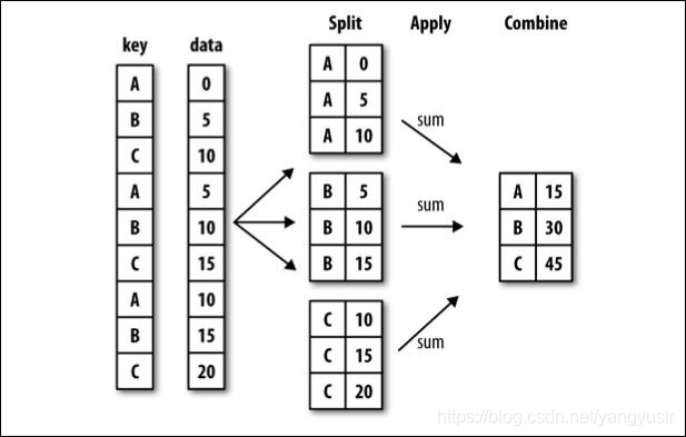
df.groupby(by=“columns_name”)
dict_obj = {
‘key1’ : [‘a’, ‘b’, ‘a’, ‘b’,‘a’, ‘b’, ‘a’, ‘a’],
‘key2’ : [‘one’, ‘one’, ‘two’, ‘three’,‘two’, ‘two’, ‘one’, ‘three’],
‘data1’: np.arange(8),
‘data2’: np.arange(8)
}
# 分组聚合
import pandas as pd
import numpy as np


dict_obj = {
    'key1': ['a', 'b', 'a', 'b', 'a', 'b', 'a', 'a'],
    'key2': ['one', 'one', 'two', 'three', 'two', 'two', 'one', 'three'],
    'data1': np.arange(8),
    'data2': np.arange(8)
}
df = pd.DataFrame(dict_obj)
print(df)
'''
  key1   key2  data1  data2
0    a    one      0      0
1    b    one      1      1
2    a    two      2      2
3    b  three      3      3
4    a    two      4      4
5    b    two      5      5
6    a    one      6      6
7    a  three      7      7
'''
# 分组 groupby
df.groupby(by="key1")
print(df.groupby(by="key1"))  # <pandas.core.groupby.generic.DataFrameGroupBy object at 0x0000000002CB9208>
for i in df.groupby(by="key1"):
    print(i)
'''
('a',   key1   key2  data1  data2
0    a    one      0      0
2    a    two      2      2
4    a    two      4      4
6    a    one      6      6
7    a  three      7      7)
('b',   key1   key2  data1  data2
1    b    one      1      1
3    b  three      3      3
5    b    two      5      5)
'''
print(df.groupby(by="key1").mean())  # 求平均值,key2不是数字类型直接忽略掉
'''
      data1  data2
key1
a       3.8    3.8
b       3.0    3.0'''
print(df.groupby(by="key1").sum())  # 求和,key2不是数字类型直接忽略掉
'''
      data1  data2
key1
a        19     19
b         9      9'''
print(df.groupby(by="key1").count())  # 记录个数
'''
      key2  data1  data2
key1
a        5      5      5
b        3      3      3'''
- 练习
现在我们有一组关于全球星巴克店铺的统计数据,如果我想知道美国的星巴克数量和中国的哪个多,或者我想知道中国每个省份星巴克的数量的情况,那么应该怎么办?
# 现在我们有一组关于全球星巴克店铺的统计数据,如果我想知道美国的星巴克数量和
# 中国的哪个多,或者我想知道中国每个省份星巴克的数量的情况,那么应该怎么办?
# 思路:根据国家分组,统计每个国家的总数进行对比,取出中国的数据,按省份分组统计每个省份的总数进行对比
import numpy as np
import pandas as pd

file_path = './starbucks_store_worldwide.csv'
df = pd.read_csv(file_path)
print(df.info())
'''
<class 'pandas.core.frame.DataFrame'>
RangeIndex: 25600 entries, 0 to 25599
Data columns (total 13 columns):
 #   Column          Non-Null Count  Dtype
---  ------          --------------  -----
 0   Brand           25600 non-null  object
 1   Store Number    25600 non-null  object
 2   Store Name      25600 non-null  object
 3   Ownership Type  25600 non-null  object
 4   Street Address  25598 non-null  object
 5   City            25585 non-null  object
 6   State/Province  25600 non-null  object
 7   Country         25600 non-null  object
 8   Postcode        24078 non-null  object
 9   Phone Number    18739 non-null  object
 10  Timezone        25600 non-null  object
 11  Longitude       25599 non-null  float64
 12  Latitude        25599 non-null  float64
dtypes: float64(2), object(11)
memory usage: 2.5+ MB
None'''
print(df.head())
'''
       Brand  Store Number  ... Longitude Latitude
0  Starbucks  47370-257954  ...      1.53    42.51
1  Starbucks  22331-212325  ...     55.47    25.42
2  Starbucks  47089-256771  ...     55.47    25.39
3  Starbucks  22126-218024  ...     54.38    24.48
4  Starbucks  17127-178586  ...     54.54    24.51
'''
pd.set_option('display.max_rows', 10)
pd.set_option('display.max_columns', 13)
print(df)
'''
                        City State/Province Country Postcode  Phone Number
0           Andorra la Vella              7      AD    AD500     376818720
1                      Ajman             AJ      AE      NaN           NaN
2                      Ajman             AJ      AE      NaN           NaN
3                  Abu Dhabi             AZ      AE      NaN           NaN
4                  Abu Dhabi             AZ      AE      NaN           NaN
...                      ...            ...     ...      ...           ...
25595  Thành Phố Hồ Chí Minh             SG      VN    70000  08 3824 4668
25596  Thành Phố Hồ Chí Minh             SG      VN    70000  08 5413 8292
25597           Johannesburg             GT      ZA     2194   27873500159
25598                 Menlyn             GT      ZA      181           NaN
25599                Midrand             GT      ZA     1682   27873500215

                             Timezone  Longitude  Latitude
0             GMT+1:00 Europe/Andorra       1.53     42.51
1                GMT+04:00 Asia/Dubai      55.47     25.42
2                GMT+04:00 Asia/Dubai      55.47     25.39
3                GMT+04:00 Asia/Dubai      54.38     24.48
4                GMT+04:00 Asia/Dubai      54.54     24.51
...                               ...        ...       ...
25595          GMT+000000 Asia/Saigon     106.70     10.78
25596          GMT+000000 Asia/Saigon     106.71     10.72
25597  GMT+000000 Africa/Johannesburg      28.04    -26.15
25598  GMT+000000 Africa/Johannesburg      28.28    -25.79
25599  GMT+000000 Africa/Johannesburg      28.11    -26.02

[25600 rows x 13 columns]
'''
grouped = df.groupby(by='Country').count()['Brand']
print(type(grouped))  # <class 'pandas.core.series.Series'>
print(grouped)
'''
AD        1
AE      144
AR      108
AT       18
AU       22
      ...
TT        3
TW      394
US    13608
VN       25
ZA        3
Name: Brand, Length: 73, dtype: int64'''
us_count = grouped['US']  # us_count = grouped.loc['US']也可以
print(us_count)  # 13608
cn_count = grouped['CN']  # cn_count = grouped.loc['CN']也可以
print(cn_count)  # 2734
print("美国的星巴克总数位%s,中国的星巴克为%s" % (us_count, cn_count))
'''美国的星巴克总数位13608,中国的星巴克为2734'''

# 布尔索引
china_data = df[df['Country'] == 'CN']
print(china_data)
'''
          Brand  Store Number           Store Name Ownership Type
2091  Starbucks  22901-225145            北京西站第一咖啡店  Company Owned
2092  Starbucks  32320-116537              北京华宇时尚店  Company Owned
2093  Starbucks  32447-132306           北京蓝色港湾圣拉娜店  Company Owned
2094  Starbucks  17477-161286           北京太阳宫凯德嘉茂店  Company Owned
2095  Starbucks  24520-237564              北京东三环北店  Company Owned
...         ...           ...                  ...            ...
4820  Starbucks  17872-186929                Sands       Licensed
4821  Starbucks  24126-235784              Wynn II       Licensed
4822  Starbucks  28490-242269      Wynn Palace BOH       Licensed
4823  Starbucks  22210-218665  Sands Cotai Central       Licensed
4824  Starbucks  17108-179449          One Central       Licensed

                                         Street Address   City State/Province
2091                          丰台区, 北京西站通廊7-1号, 中关村南大街2号    北京市             11
2092          海淀区, 数码大厦B座华宇时尚购物中心内, 蓝色港湾国际商区1座C1-3单元首层、    北京市             11
2093                朝阳区朝阳公园路6号, 二层C1-3单元及二层阳台, 太阳宫中路12号    北京市             11
2094                  朝阳区, 太阳宫凯德嘉茂一层01-44/45号, 东三环北路27号    北京市             11
2095                      朝阳区, 嘉铭中心大厦A座B1层024商铺, 金融大街7号    北京市             11
...                                                 ...    ...            ...
4820  Portion of Shop 04, Ground Floor, Sands, Largo...  Macau             92
4821             Wynn Macau, Rua Cidada de Sintra, NAPE  Macau             92
4822       Employee Entrance Outlet, Wynn Cotai, Resort  Macau             92
4823  Shop K201 & K202, Level 02, Parcela 5&6, Estra...  Macau             92
4824                       Promenade Rd, Open Area, 2/F  Macau             92

     Country Postcode   Phone Number                Timezone  Longitude
2091      CN   100073            NaN  GMT+08:00 Asia/Beijing     116.32
2092      CN   100086   010-51626616  GMT+08:00 Asia/Beijing     116.32
2093      CN   100020   010-59056343  GMT+08:00 Asia/Beijing     116.47
2094      CN   100028   010-84150945  GMT+08:00 Asia/Beijing     116.45
2095      CN      NaN            NaN  GMT+08:00 Asia/Beijing     116.46
...      ...      ...            ...                     ...        ...
4820      CN      NaN  (853)28782773  GMT+08:00 Asia/Beijing     113.55
4821      CN      NaN    85328723516  GMT+08:00 Asia/Beijing     113.55
4822      CN      NaN            NaN  GMT+08:00 Asia/Beijing     113.54
4823      CN      NaN    85328853439  GMT+08:00 Asia/Beijing     113.56
4824      CN      NaN            NaN  GMT+08:00 Asia/Beijing     113.55

      Latitude
2091     39.90
2092     39.97
2093     39.95
2094     39.97
2095     39.93
...        ...
4820     22.19
4821     22.19
4822     22.20
4823     22.15
4824     22.19

[2734 rows x 13 columns]
'''
china_province_data = china_data.groupby(by='State/Province').count()
print(china_province_data['Brand'])
'''
State/Province
11    236
12     58
13     24
14      8
15      8
     ...
62      3
63      3
64      2
91    162
92     13
Name: Brand, Length: 31, dtype: int64'''
- DataFrameGroupBy对象方法
方法 说明
count 分组中非NA值的数量
sum 非NA值的和
mean 非NA值的平均值
min,max 非NA值的最小值和最大值
4.索引和复合索引
- 简单的索引操作: t.index
- 指定index: t.index = [‘a’,‘b’,‘c’]
- 重新设置index : t.reindex([“a”,“e”])
- 指定某一列作为index : t.set_index(“M”,drop=False)
- 返回index的唯一值: t.set_index(“M”).index.unique()
- 设置两个索引的时候会是什么样子呢?
- 示例
# 索引和复合索引
import numpy as np
import pandas as pd

t1 = pd.DataFrame(np.arange(12).reshape(3, 4), index=list('ABC'), columns=list('WXYZ'))
print(t1)
'''
   W  X   Y   Z
A  0  1   2   3
B  4  5   6   7
C  8  9  10  11'''
print(t1.index)  # Index(['A', 'B', 'C'], dtype='object')
# 重置索引
print(t1.reindex(['a','e']))
'''
    W   X   Y   Z
a NaN NaN NaN NaN
e NaN NaN NaN NaN'''
print(t1.reindex(['A','e']))
'''
     W    X    Y    Z
A  0.0  1.0  2.0  3.0
e  NaN  NaN  NaN  NaN'''
# 指定某一列作为索引
print(t1.set_index('W'))  # 默认删除W列,以W作为行索引
'''
   X   Y   Z
W
0  1   2   3
4  5   6   7
8  9  10  11'''
print(t1.set_index('W',drop=False))  # 不删除W列,以W作为行索引
'''
   W  X   Y   Z
W
0  0  1   2   3
4  4  5   6   7
8  8  9  10  11'''
# 返回index的唯一值: t.set_index("M").index.unique()
print(t1.set_index('W').index)
'''Int64Index([0, 4, 8], dtype='int64', name='W')'''
print(t1.set_index('W').index.unique())
'''Int64Index([0, 4, 8], dtype='int64', name='W')'''
t1.loc['B','W'] = 8
print(t1)
'''
   W  X   Y   Z
A  0  1   2   3
B  8  5   6   7
C  8  9  10  11'''
print(t1.set_index('W').index.unique())
'''Int64Index([0, 8], dtype='int64', name='W')'''
# 设置两个索引  复合索引
t2 = pd.DataFrame(np.arange(12).reshape(3, 4), index=list('ABC'), columns=list('WXYZ'))
print(t2)
'''
   W  X   Y   Z
A  0  1   2   3
B  4  5   6   7
C  8  9  10  11'''
print(t2.set_index(['W','X']))
'''
      Y   Z
W X
0 1   2   3
4 5   6   7
8 9  10  11'''
print(type(t2.set_index(['W','X'])))  # <class 'pandas.core.frame.DataFrame'>
Series复合索引
a = pd.DataFrame({‘a’: range(7),‘b’: range(7, 0, -1),‘c’: [‘one’,‘one’,‘one’,‘two’,‘two’,‘two’, ‘two’],‘d’:
list(“hjklmno”)})
设置c,d为索引
# 索引和复合索引
import numpy as np
import pandas as pd

a = pd.DataFrame({'a': range(7), 'b': range(7, 0, -1), 'c': ['one', 'one', 'one', 'two', 'two', 'two', 'two'], 'd':
    list("hjklmno")})
print(type(a))  # <class 'pandas.core.frame.DataFrame'>
print(a)
'''
   a  b    c  d
0  0  7  one  h
1  1  6  one  j
2  2  5  one  k
3  3  4  two  l
4  4  3  two  m
5  5  2  two  n
6  6  1  two  o'''
b = a.set_index(['c','d'])
print(b)
'''
       a  b
c   d
one h  0  7
    j  1  6
    k  2  5
two l  3  4
    m  4  3
    n  5  2
    o  6  1
'''
print(b.loc['one'])
'''
   a  b
d
h  0  7
j  1  6
k  2  5'''
print(b.loc['one'].loc['j'])
'''
a    1
b    6
Name: j, dtype: int64'''
print(b.loc['one'].loc['j']['a'])  # 1
c = b['a']
print(type(c))  # <class 'pandas.core.series.Series'>
print(c)
'''
c    d
one  h    0
     j    1
     k    2
two  l    3
     m    4
     n    5
     o    6
Name: a, dtype: int64'''
print(c['one']['j'])  # 1
print(c['one','j'])  # 1
设置d,c为索引
# 索引和复合索引
import numpy as np
import pandas as pd

a = pd.DataFrame({'a': range(7), 'b': range(7, 0, -1), 'c': ['one', 'one', 'one', 'two', 'two', 'two', 'two'], 'd':
    list("hjklmno")})
print(type(a))  # <class 'pandas.core.frame.DataFrame'>
print(a)
'''
   a  b    c  d
0  0  7  one  h
1  1  6  one  j
2  2  5  one  k
3  3  4  two  l
4  4  3  two  m
5  5  2  two  n
6  6  1  two  o'''
b = a.set_index(['d','c'])
print(b)
'''
       a  b
d c
h one  0  7
j one  1  6
k one  2  5
l two  3  4
m two  4  3
n two  5  2
o two  6  1
'''
print(b.loc['j'])
'''
     a  b
c
one  1  6'''
print(b.loc['j'].loc['one'])
'''
a    1
b    6
Name: one, dtype: int64'''
print(b.loc['j'].loc['one']['a'])  # 1
print(b.loc['j'].loc['one','a'])  # 1
# 复合索引交换
print(b.swaplevel())
'''
       a  b
c   d
one h  0  7
    j  1  6
    k  2  5
two l  3  4
    m  4  3
    n  5  2
    o  6  1'''
DateFrame复合索引
# 索引和复合索引
import numpy as np
import pandas as pd

a = pd.DataFrame({'a': range(7), 'b': range(7, 0, -1), 'c': ['one', 'one', 'one', 'two', 'two', 'two', 'two'], 'd':
    list("hjklmno")})
print(type(a))  # <class 'pandas.core.frame.DataFrame'>
print(a)
'''
   a  b    c  d
0  0  7  one  h
1  1  6  one  j
2  2  5  one  k
3  3  4  two  l
4  4  3  two  m
5  5  2  two  n
6  6  1  two  o'''
b = a.set_index(['c','d'])
print(b)
'''
       a  b
c   d
one h  0  7
    j  1  6
    k  2  5
two l  3  4
    m  4  3
    n  5  2
    o  6  1
'''
# 从外层开始取值
print(b.loc['one'].loc['j','b'])  # 6
# 从内层开始取值
print(b.swaplevel().loc['j'].loc['one','b'])  # 6
5.练习
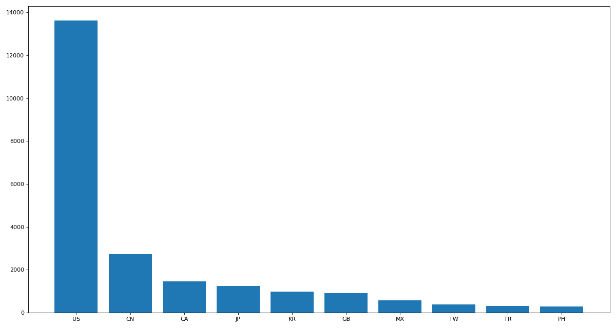
1.使用matplotlib呈现出店铺总数排名前10的国家
# # 1.使用matplotlib呈现出店铺总数排名前10的国家  # sort_values  groupby
import numpy as np
import pandas as pd
from matplotlib import pyplot as plt

file_path = './starbucks_store_worldwide.csv'
df = pd.read_csv(file_path)
print(df.info())
'''
<class 'pandas.core.frame.DataFrame'>
RangeIndex: 25600 entries, 0 to 25599
Data columns (total 13 columns):
 #   Column          Non-Null Count  Dtype
---  ------          --------------  -----
 0   Brand           25600 non-null  object
 1   Store Number    25600 non-null  object
 2   Store Name      25600 non-null  object
 3   Ownership Type  25600 non-null  object
 4   Street Address  25598 non-null  object
 5   City            25585 non-null  object
 6   State/Province  25600 non-null  object
 7   Country         25600 non-null  object
 8   Postcode        24078 non-null  object
 9   Phone Number    18739 non-null  object
 10  Timezone        25600 non-null  object
 11  Longitude       25599 non-null  float64
 12  Latitude        25599 non-null  float64
dtypes: float64(2), object(11)
memory usage: 2.5+ MB
None'''
data = df.groupby(by='Country').count()
print(data.head(3))
'''
         Brand  Store Number  Store Name  ...  Timezone  Longitude  Latitude
Country                                   ...
AD           1             1           1  ...         1          1         1
AE         144           144         144  ...       144        144       144
AR         108           108         108  ...       108        108       108

[3 rows x 12 columns]'''
data_sort = data.sort_values(by='Brand', ascending=False)[0:10]  # 倒序
print(data_sort['Brand'])
# data = df.groupby(by='Country').count()['Brand'].sort_values(ascending=False)[0:10]
# print(data)  # 这样写也可以
'''
Country
US    13608
CN     2734
CA     1468
JP     1237
KR      993
GB      901
MX      579
TW      394
TR      326
PH      298
Name: Brand, dtype: int64'''
x = data_sort['Brand'].index
y = data_sort['Brand'].values

# 设置图片大小
plt.figure(figsize=(15, 8), dpi=80)
# 直方图
plt.bar(x, y)
plt.show()
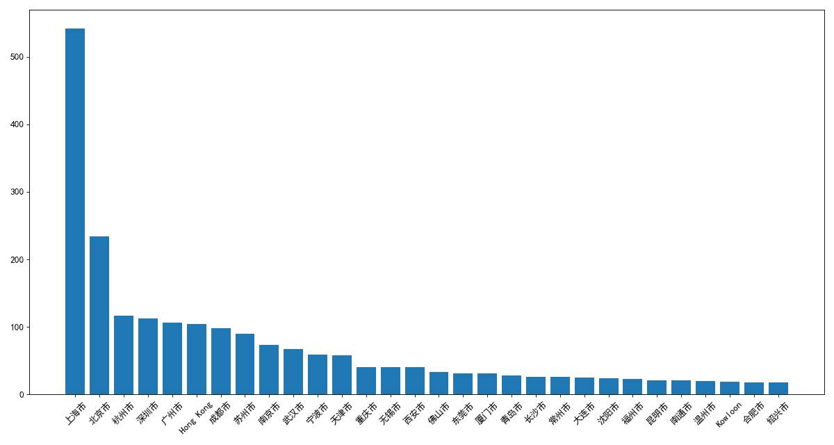
2.使用matplotlib呈现出中国每个城市的店铺数量
# 2.使用matplotlib呈现出中国每个城市的店铺数量

import pandas as pd
from matplotlib import pyplot as plt
import matplotlib

font = {
    'family': 'SimHei',
    'weight': 'bold',
    'size': 12
}
matplotlib.rc("font", **font)

file_path = './starbucks_store_worldwide.csv'
df = pd.read_csv(file_path)
# print(df.info())
'''
 #   Column          Non-Null Count  Dtype
---  ------          --------------  -----
 0   Brand           25600 non-null  object
 1   Store Number    25600 non-null  object
 2   Store Name      25600 non-null  object
 3   Ownership Type  25600 non-null  object
 4   Street Address  25598 non-null  object
 5   City            25585 non-null  object
 6   State/Province  25600 non-null  object
 7   Country         25600 non-null  object
 8   Postcode        24078 non-null  object
 9   Phone Number    18739 non-null  object
 10  Timezone        25600 non-null  object
 11  Longitude       25599 non-null  float64
 12  Latitude        25599 non-null  float64
dtypes: float64(2), object(11)
memory usage: 2.5+ MB
None'''
df = df[df['Country'] == 'CN']
# print(df.head(3))
'''
          Brand  Store Number  ... Longitude Latitude
2091  Starbucks  22901-225145  ...    116.32    39.90
2092  Starbucks  32320-116537  ...    116.32    39.97
2093  Starbucks  32447-132306  ...    116.47    39.95

[3 rows x 13 columns]'''
data = df.groupby(by='City').count()['Brand'].sort_values(ascending=False)[0:30]
x = data.index
y = data.values

# 设置图片大小
plt.figure(figsize=(15, 8), dpi=80)
# 直方图
plt.bar(x, y)
# 设置x轴刻度
plt.xticks(rotation=45)
plt.show()
三、pandas中的时间序列
1.时间范围
时间范围
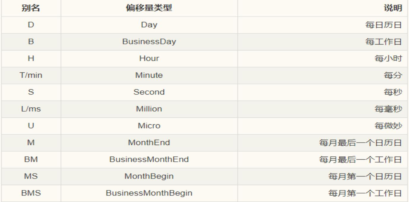
pd.date_range(start=None, end=None, periods=None, freq=‘D’)
periods 时间范围的个数
freq 频率,以天为单位还是以月为单位
关于频率的更多缩写
- 示例
# 时间序列
import pandas as pd

d = pd.date_range(start='20210101', end='20210201')
print(d)  # freq='D' 频率默认是天
'''DatetimeIndex(['2021-01-01', '2021-01-02', '2021-01-03', '2021-01-04',
               '2021-01-05', '2021-01-06', '2021-01-07', '2021-01-08',
               '2021-01-09', '2021-01-10', '2021-01-11', '2021-01-12',
               '2021-01-13', '2021-01-14', '2021-01-15', '2021-01-16',
               '2021-01-17', '2021-01-18', '2021-01-19', '2021-01-20',
               '2021-01-21', '2021-01-22', '2021-01-23', '2021-01-24',
               '2021-01-25', '2021-01-26', '2021-01-27', '2021-01-28',
               '2021-01-29', '2021-01-30', '2021-01-31', '2021-02-01'],
              dtype='datetime64[ns]', freq='D')'''
m = pd.date_range(start='20210101', end='20211231',freq='M')  # 频率是1月
print(m)
'''
DatetimeIndex(['2021-01-31', '2021-02-28', '2021-03-31', '2021-04-30',
               '2021-05-31', '2021-06-30', '2021-07-31', '2021-08-31',
               '2021-09-30', '2021-10-31', '2021-11-30', '2021-12-31'],
              dtype='datetime64[ns]', freq='M')'''
d10 = pd.date_range(start='20210101', end='20210201',freq='10D')
print(d10)  # freq='10D' 频率是10天
'''
DatetimeIndex(['2021-01-01', '2021-01-11', '2021-01-21', '2021-01-31'], dtype='datetime64[ns]', freq='10D')'''
d3 = pd.date_range(start='20210101', end='20210201',freq='3D')
print(d3)  # freq='10D' 频率是3天
'''
DatetimeIndex(['2021-01-01', '2021-01-04', '2021-01-07', '2021-01-10',
               '2021-01-13', '2021-01-16', '2021-01-19', '2021-01-22',
               '2021-01-25', '2021-01-28', '2021-01-31'],
              dtype='datetime64[ns]', freq='3D')'''
d3 = pd.date_range(start='20210101', periods=5, freq='3D')
print(d3)  # freq='10D' 频率是3天  periods和end不要同时用
'''
DatetimeIndex(['2021-01-01', '2021-01-04', '2021-01-07', '2021-01-10',
               '2021-01-13'],
              dtype='datetime64[ns]', freq='3D')'''
2.DataFrame中使用时间序列
index=pd.date_range(“20190101”,periods=10)
df = pd.DataFrame(np.arange(10),index=index) 作为行索引
df = pd.DataFrame(np.arange(10).reshape(1,10),columns=index) 作为列索引
- 示例
# 使用时间序列
import pandas as pd
import numpy as np

# 时间序列当行索引
dindex = pd.date_range(start='20210101', periods=10)
df = pd.DataFrame(np.arange(10),index=dindex)
print(df)
'''
            0
2021-01-01  0
2021-01-02  1
2021-01-03  2
2021-01-04  3
2021-01-05  4
2021-01-06  5
2021-01-07  6
2021-01-08  7
2021-01-09  8
2021-01-10  9
'''
# 时间序列当列索引
d_index = pd.date_range(start='20210101', periods=10)
df1 = pd.DataFrame(np.arange(10).reshape(1,10),columns=d_index)
print(df1)
'''
   2021-01-01  2021-01-02  2021-01-03  ...  2021-01-08  2021-01-09  2021-01-10
0           0           1           2  ...           7           8           9

[1 rows x 10 columns]'''
3.pandas重采样
- 重采样:指的是将时间序列从一个频率转化为另一个频率进行处理的过程,将高频率数据转化为低频率数据为降采样,低频率转化为高频率为升采样
- pandas提供了一个resample的方法来帮助我们实现频率转化
- 示例
# 使用时间序列
import pandas as pd
import numpy as np

dindex = pd.date_range(start='2021-01-01',end='2021-02-24')
t = pd.DataFrame(np.arange(55).reshape(55,1),index=dindex)
print(t)
'''
             0
2021-01-01   0
2021-01-02   1
2021-01-03   2
2021-01-04   3
2021-01-05   4
2021-01-06   5
2021-01-07   6
2021-01-08   7
2021-01-09   8
2021-01-10   9
2021-01-11  10
2021-01-12  11
2021-01-13  12
2021-01-14  13
2021-01-15  14
2021-01-16  15
2021-01-17  16
2021-01-18  17
2021-01-19  18
2021-01-20  19
2021-01-21  20
2021-01-22  21
2021-01-23  22
2021-01-24  23
2021-01-25  24
2021-01-26  25
2021-01-27  26
2021-01-28  27
2021-01-29  28
2021-01-30  29
2021-01-31  30
2021-02-01  31
2021-02-02  32
2021-02-03  33
2021-02-04  34
2021-02-05  35
2021-02-06  36
2021-02-07  37
2021-02-08  38
2021-02-09  39
2021-02-10  40
2021-02-11  41
2021-02-12  42
2021-02-13  43
2021-02-14  44
2021-02-15  45
2021-02-16  46
2021-02-17  47
2021-02-18  48
2021-02-19  49
2021-02-20  50
2021-02-21  51
2021-02-22  52
2021-02-23  53
2021-02-24  54
'''
print(t.resample('M').mean())
'''
               0
2021-01-31  15.0
2021-02-28  42.5'''
print(t.resample('10D').mean())
'''
               0
2021-01-01   4.5
2021-01-11  14.5
2021-01-21  24.5
2021-01-31  34.5
2021-02-10  44.5
2021-02-20  52.0'''
4.练习
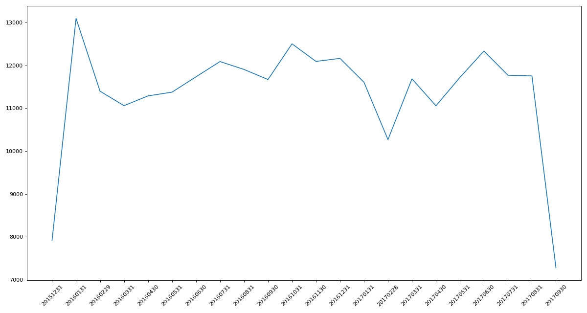
练习1:统计出911数据中不同月份的电话次数
# 练习1:统计出911数据中不同月份的电话次数
import pandas as pd
from matplotlib import pyplot as plt

file_path = './911.csv'
df = pd.read_csv(file_path)
pd.set_option('display.max_rows', 30)
pd.set_option('display.max_columns', 9)
# print(df.info())
'''
<class 'pandas.core.frame.DataFrame'>
RangeIndex: 249737 entries, 0 to 249736
Data columns (total 9 columns):
 #   Column     Non-Null Count   Dtype
---  ------     --------------   -----
 0   lat        249737 non-null  float64
 1   lng        249737 non-null  float64
 2   desc       249737 non-null  object
 3   zip        219391 non-null  float64
 4   title      249737 non-null  object
 5   timeStamp  249737 non-null  object
 6   twp        249644 non-null  object
 7   addr       249737 non-null  object
 8   e          249737 non-null  int64
dtypes: float64(3), int64(1), object(5)
memory usage: 17.1+ MB
None
'''
# print(df['timeStamp'])
'''0         2015-12-10 17:10:52
                 ...
249736    2017-09-20 19:42:29
Name: timeStamp, Length: 249737, dtype: object'''
df['timeStamp'] = pd.to_datetime(df['timeStamp'])  # 把时间字符串转为索引
# print(df['timeStamp'])
'''
0        2015-12-10 17:10:52
                 ...
249736   2017-09-20 19:42:29
Name: timeStamp, Length: 249737, dtype: datetime64[ns]'''
df.set_index('timeStamp', inplace=True)
# print(df)
'''
                           lat        lng
timeStamp
2015-12-10 17:10:52  40.297876 -75.581294
...                        ...        ...
2017-09-20 19:42:29  40.095206 -75.410735

                                                                  desc
timeStamp
2015-12-10 17:10:52  REINDEER CT & DEAD END;  NEW HANOVER; Station ...
...                                                                ...
2017-09-20 19:42:29  1ST AVE & MOORE RD; UPPER MERION; 2017-09-20 @...

                         zip                        title           twp
timeStamp
2015-12-10 17:10:52  19525.0       EMS: BACK PAINS/INJURY   NEW HANOVER
...                      ...                          ...           ...
2017-09-20 19:42:29  19406.0  Traffic: VEHICLE ACCIDENT -  UPPER MERION

                                       addr  e
timeStamp
2015-12-10 17:10:52  REINDEER CT & DEAD END  1
...                                     ... ..
2017-09-20 19:42:29      1ST AVE & MOORE RD  1

[249737 rows x 8 columns]
'''
count_by_month = df.resample('M').count()['lat']
print(count_by_month)
'''
timeStamp
2015-12-31     7916
2016-01-31    13096
2016-02-29    11396
2016-03-31    11059
2016-04-30    11287
2016-05-31    11374
2016-06-30    11732
2016-07-31    12088
2016-08-31    11904
2016-09-30    11669
2016-10-31    12502
2016-11-30    12091
2016-12-31    12162
2017-01-31    11605
2017-02-28    10267
2017-03-31    11684
2017-04-30    11056
2017-05-31    11719
2017-06-30    12333
2017-07-31    11768
2017-08-31    11753
2017-09-30     7276
Freq: M, Name: lat, dtype: int64
'''
# 绘制折线图分析变化趋势
x = count_by_month.index
y = count_by_month.values
x = [i.strftime("%Y%m%d") for i in x]  # 转化为时间日期格式。
plt.figure(figsize=(15, 8), dpi=80)
plt.plot(range(len(x)), y)
plt.xticks(range(len(x)), x, rotation=45)
plt.show()
https://www.kaggle.com/uciml/pm25-data-for-five-chinese-cities
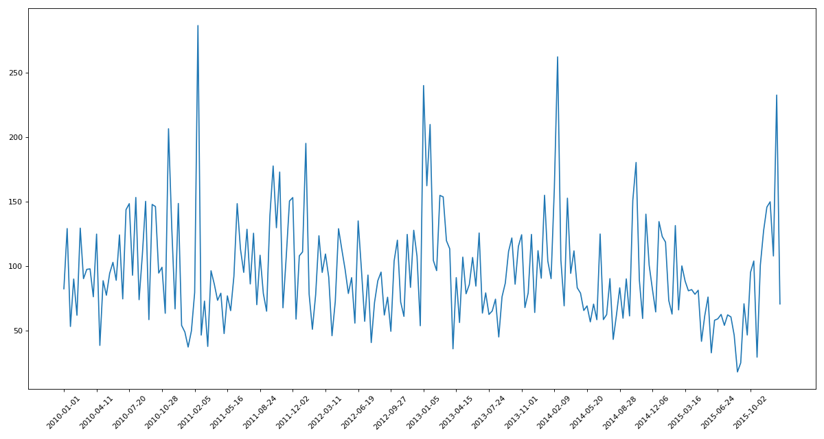
练习2现在我们有北上广、深圳、和沈阳5个城市空气质量数据,请绘制出5个城市的PM2.5随时间的变化情况
数据来源:https://www.kaggle.com/uciml/pm25-data-for-five-chinese-cities
观察这组数据中的时间结构,并不是字符串,这个时候我们应该怎么办?
之前所学习的DatetimeIndex可以理解为时间戳
那么现在我们要学习的PeriodIndex可以理解为时间段
periods = pd.PeriodIndex(year=df[“year”],month=df[“month”],day=df[“day”],hour=df[“hour”],freq=“H”)
那么如果给这个时间段降采样呢?
data = df.set_index(periods).resample(“10D”).mean()
# 现在我们有北上广、深圳、和沈阳5个城市空气质量数据,请绘制出5个城市的PM2.5随时间的变化情况
import pandas as pd
from matplotlib import pyplot as plt

df = pd.read_csv('./PM2.5/BeijingPM20100101_20151231.csv')
# print(df.info())
'''
<class 'pandas.core.frame.DataFrame'>
RangeIndex: 52584 entries, 0 to 52583
Data columns (total 18 columns):
 #   Column           Non-Null Count  Dtype
---  ------           --------------  -----
 0   No               52584 non-null  int64
 1   year             52584 non-null  int64
 2   month            52584 non-null  int64
 3   day              52584 non-null  int64
 4   hour             52584 non-null  int64
 5   season           52584 non-null  int64
 6   PM_Dongsi        25052 non-null  float64
 7   PM_Dongsihuan    20508 non-null  float64
 8   PM_Nongzhanguan  24931 non-null  float64
 9   PM_US Post       50387 non-null  float64
 10  DEWP             52579 non-null  float64
 11  HUMI             52245 non-null  float64
 12  PRES             52245 non-null  float64
 13  TEMP             52579 non-null  float64
 14  cbwd             52579 non-null  object
 15  Iws              52579 non-null  float64
 16  precipitation    52100 non-null  float64
 17  Iprec            52100 non-null  float64
dtypes: float64(11), int64(6), object(1)
memory usage: 7.2+ MB
None'''
pd.set_option('display.max_rows', 30)
pd.set_option('display.max_columns', 18)
# print(df.head())
'''
   No  year  month  day  hour  season  PM_Dongsi  PM_Dongsihuan
0   1  2010      1    1     0       4        NaN            NaN
1   2  2010      1    1     1       4        NaN            NaN
2   3  2010      1    1     2       4        NaN            NaN
3   4  2010      1    1     3       4        NaN            NaN
4   5  2010      1    1     4       4        NaN            NaN

   PM_Nongzhanguan  PM_US Post  DEWP  HUMI    PRES  TEMP cbwd    Iws
0              NaN         NaN -21.0  43.0  1021.0 -11.0   NW   1.79
1              NaN         NaN -21.0  47.0  1020.0 -12.0   NW   4.92
2              NaN         NaN -21.0  43.0  1019.0 -11.0   NW   6.71
3              NaN         NaN -21.0  55.0  1019.0 -14.0   NW   9.84
4              NaN         NaN -20.0  51.0  1018.0 -12.0   NW  12.97

   precipitation  Iprec
0            0.0    0.0
1            0.0    0.0
2            0.0    0.0
3            0.0    0.0
4            0.0    0.0
'''
# pd.PeriodIndex 把分开的时间字符串通过PeriodIndex的方法转换为pandas的时间类型
periods = pd.PeriodIndex(year=df["year"], month=df["month"], day=df["day"], hour=df["hour"], freq="H")
# print(periods)
'''
PeriodIndex(['2010-01-01 00:00', '2010-01-01 01:00', '2010-01-01 02:00',
             '2010-01-01 03:00', '2010-01-01 04:00', '2010-01-01 05:00',
             '2010-01-01 06:00', '2010-01-01 07:00', '2010-01-01 08:00',
             '2010-01-01 09:00',
             ...
             '2015-12-31 14:00', '2015-12-31 15:00', '2015-12-31 16:00',
             '2015-12-31 17:00', '2015-12-31 18:00', '2015-12-31 19:00',
             '2015-12-31 20:00', '2015-12-31 21:00', '2015-12-31 22:00',
             '2015-12-31 23:00'],
            dtype='period[H]', length=52584, freq='H')
'''
df['datetime'] = periods
df.set_index('datetime',inplace=True)
# print(df.head())
'''
                  No  year  month  day  hour  season  PM_Dongsi
datetime
2010-01-01 00:00   1  2010      1    1     0       4        NaN
2010-01-01 01:00   2  2010      1    1     1       4        NaN
2010-01-01 02:00   3  2010      1    1     2       4        NaN
2010-01-01 03:00   4  2010      1    1     3       4        NaN
2010-01-01 04:00   5  2010      1    1     4       4        NaN

                  PM_Dongsihuan  PM_Nongzhanguan  PM_US Post  DEWP  HUMI
datetime
2010-01-01 00:00            NaN              NaN         NaN -21.0  43.0
2010-01-01 01:00            NaN              NaN         NaN -21.0  47.0
2010-01-01 02:00            NaN              NaN         NaN -21.0  43.0
2010-01-01 03:00            NaN              NaN         NaN -21.0  55.0
2010-01-01 04:00            NaN              NaN         NaN -20.0  51.0

                    PRES  TEMP cbwd    Iws  precipitation  Iprec
datetime
2010-01-01 00:00  1021.0 -11.0   NW   1.79            0.0    0.0
2010-01-01 01:00  1020.0 -12.0   NW   4.92            0.0    0.0
2010-01-01 02:00  1019.0 -11.0   NW   6.71            0.0    0.0
2010-01-01 03:00  1019.0 -14.0   NW   9.84            0.0    0.0
2010-01-01 04:00  1018.0 -12.0   NW  12.97            0.0    0.0
'''
# 进行降采样
df = df.resample('10D').mean()
# 处理缺失数据
data = df['PM_US Post'].dropna()
# print(data)
'''
datetime
2010-01-01 23:00    129.0
2010-01-02 00:00    148.0
2010-01-02 01:00    159.0
2010-01-02 02:00    181.0
2010-01-02 03:00    138.0
                    ...
2015-12-31 19:00    133.0
2015-12-31 20:00    169.0
2015-12-31 21:00    203.0
2015-12-31 22:00    212.0
2015-12-31 23:00    235.0
Freq: H, Name: PM_US Post, Length: 50387, dtype: float64
'''
x = data.index
y = data.values
plt.figure(figsize=(15,8),dpi=80)
plt.plot(range(len(x)),y)
plt.xticks(range(0,len(x),10),list(x)[::10],rotation=45)
plt.show()
四、pandas画图
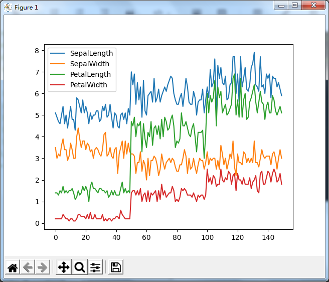
1.折线图
# pandas绘图
from matplotlib import pyplot as plt
import pandas as pd

iris_data = pd.read_csv('iris.csv')
# print(iris_data.info())
'''
<class 'pandas.core.frame.DataFrame'>
RangeIndex: 150 entries, 0 to 149
Data columns (total 5 columns):
 #   Column       Non-Null Count  Dtype
---  ------       --------------  -----
 0   SepalLength  150 non-null    float64
 1   SepalWidth   150 non-null    float64
 2   PetalLength  150 non-null    float64
 3   PetalWidth   150 non-null    float64
 4   Name         150 non-null    object
dtypes: float64(4), object(1)
memory usage: 6.0+ KB
None
'''
# 折线图
iris_data.plot()
plt.show()
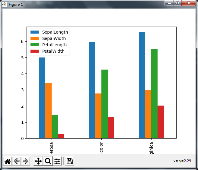
2.分组柱状图
# pandas绘图
from matplotlib import pyplot as plt
import pandas as pd

iris_data = pd.read_csv('iris.csv')
# print(iris_data.info())

# 分组柱状图
iris_data.groupby('Name').mean().plot(kind='bar')
plt.show()
2.饼图
# pandas绘图
from matplotlib import pyplot as plt
import pandas as pd

iris_data = pd.read_csv('iris.csv')
# print(iris_data.info())

# 饼图
iris_data.groupby('Name').size().plot(kind='pie',autopct='%.2f%%')
plt.show()

最后
以上就是安详鲜花最近收集整理的关于数据分析 第七讲 pandas练习 数据的合并、分组聚合、时间序列、pandas绘图数据分析 第七讲 pandas练习 数据的合并和分组聚合的全部内容,更多相关数据分析内容请搜索靠谱客的其他文章。


发表评论 取消回复