这篇文章来看一下，使用加入随机的噪声之后产生的数据进行训练，看是否能够得到期待的结果。

事前准备

训练数据使用如下方式生成：

xdata = np.linspace(0,1,100)
ydata = 2 * xdata + 1 + np.random.rand(*xdata.shape)

示例代码

liumiaocn:tensorflow liumiao$ cat basic-operation-12.py 
import tensorflow as tf
import numpy      as np
import os
import matplotlib.pyplot as plt

os.environ['TF_CPP_MIN_LOG_LEVEL'] = '2'

xdata = np.linspace(0,1,100)
ydata = 2 * xdata + 1 + np.random.rand(*xdata.shape)

print("init modole ...")
X = tf.placeholder("float",name="X")
Y = tf.placeholder("float",name="Y")
W = tf.Variable(-3., name="W")
B = tf.Variable(3., name="B")
linearmodel = tf.add(tf.multiply(X,W),B)
lossfunc = (tf.pow(Y - linearmodel, 2))
learningrate = 0.01

print("set Optimizer")
trainoperation = tf.train.GradientDescentOptimizer(learningrate).minimize(lossfunc)

sess = tf.Session()
init = tf.global_variables_initializer()
sess.run(init)

index = 1
print("caculation begins ...")
for j in range(100):
  for i in range(100):
    sess.run(trainoperation, feed_dict={X: xdata[i], Y:ydata[i]})
  if j % 10 == 0:
    print("j = %s index = %s" %(j,index))
    plt.subplot(2,5,index) 
    plt.scatter(xdata,ydata)
    labelinfo="iteration: " + str(j)
    plt.plot(xdata,B.eval(session=sess)+W.eval(session=sess)*xdata,'b',label=labelinfo)
    plt.plot(xdata,2*xdata + 1,'r',label='expected')
    plt.legend() 
    index = index + 1

print("caculation ends ...")
print("##After Caculation: ") 
print("   B: " + str(B.eval(session=sess)) + ", W : " + str(W.eval(session=sess)))

plt.show()
liumiaocn:tensorflow liumiao$

结果确认

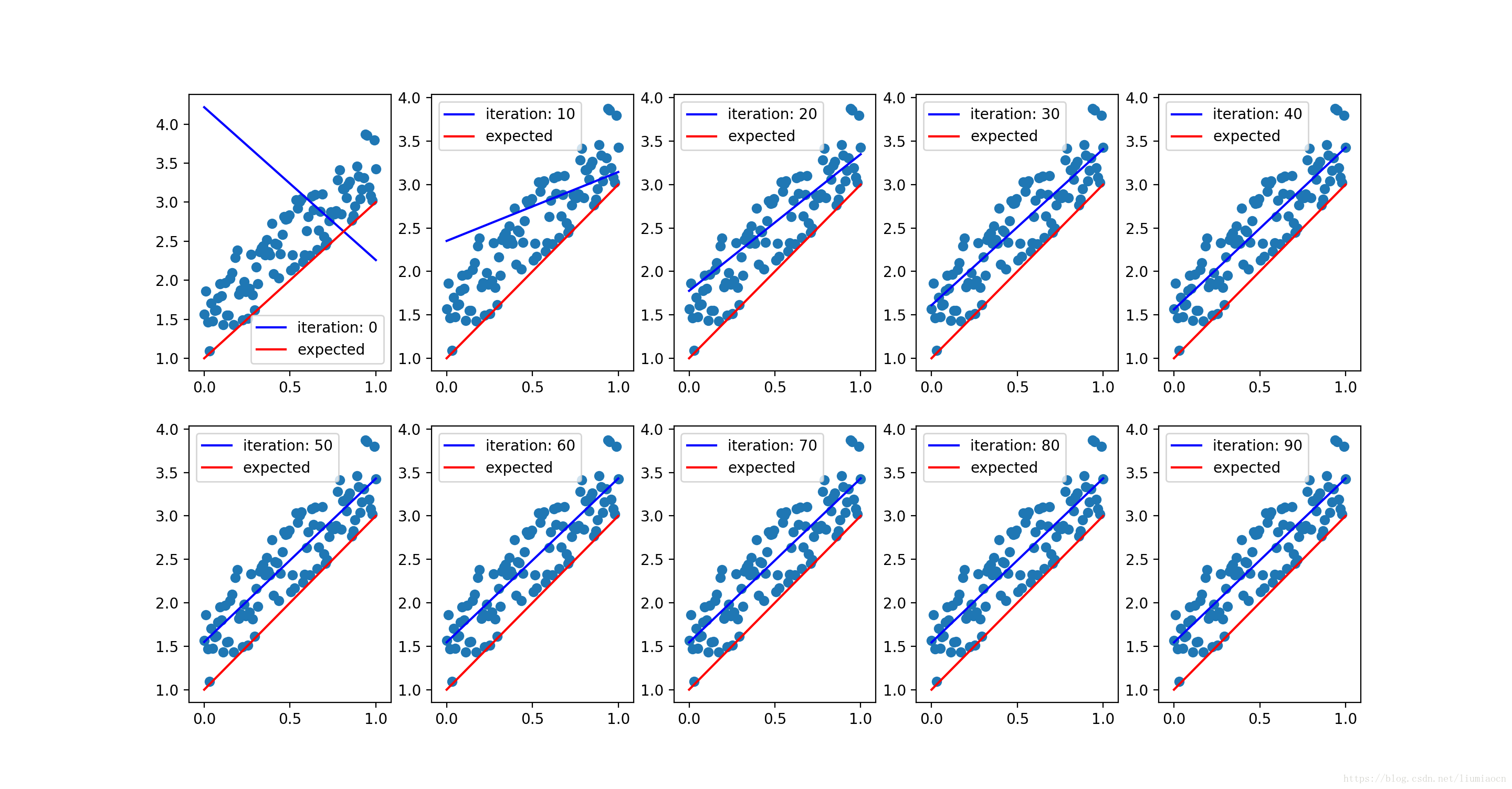
100次迭代之后的，线性模型如下：

##After Caculation: 
   B: 1.46369, W : 2.0256715

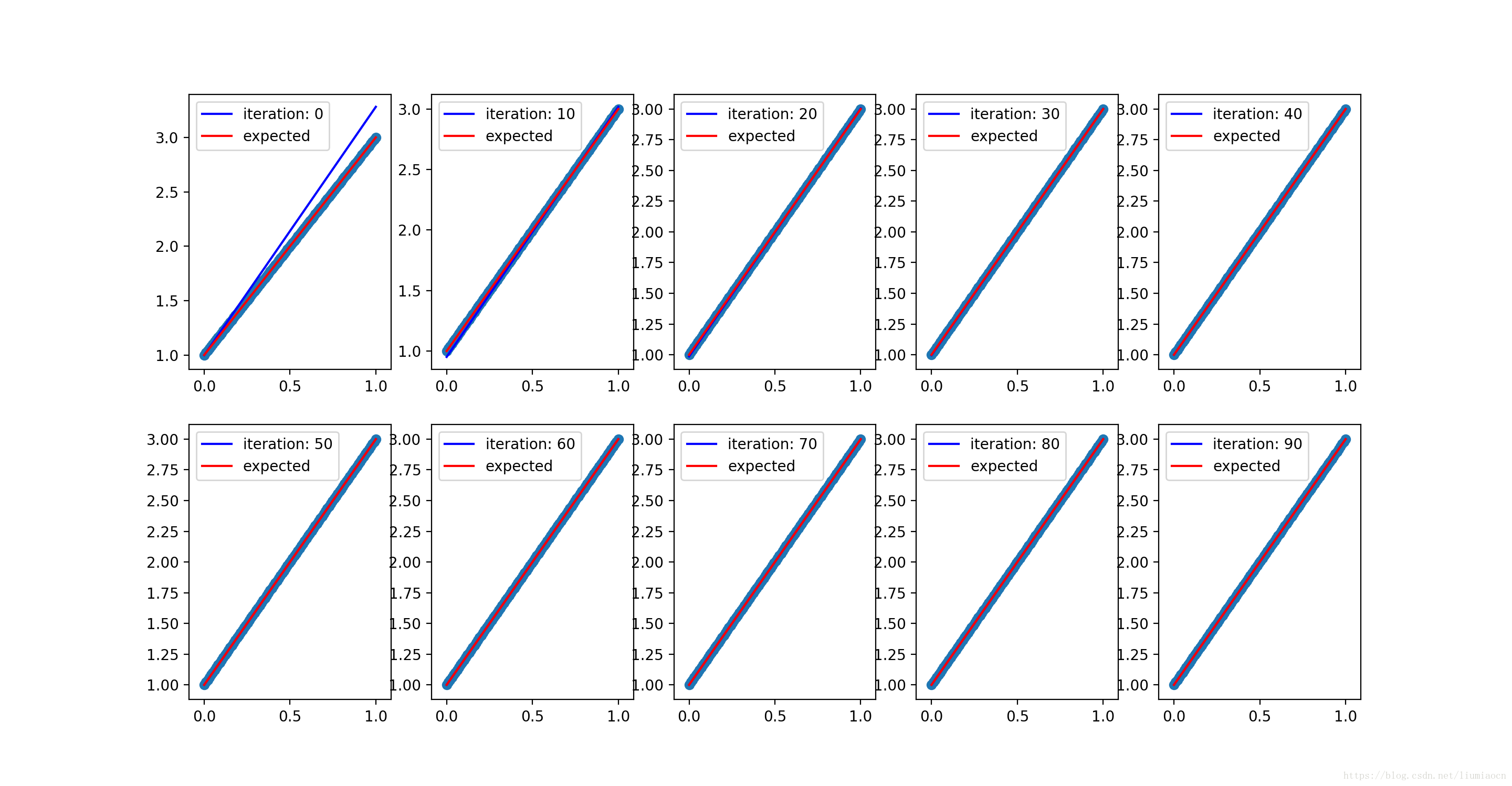
没有噪声的学习过程, 收敛的如下：

可以看到对加入噪声之后的数据，收敛的过程很好，但是偏差B没有能够得到理想的结果，把迭代增加值1000次，每100次确认一下状态，得到的结果如下：

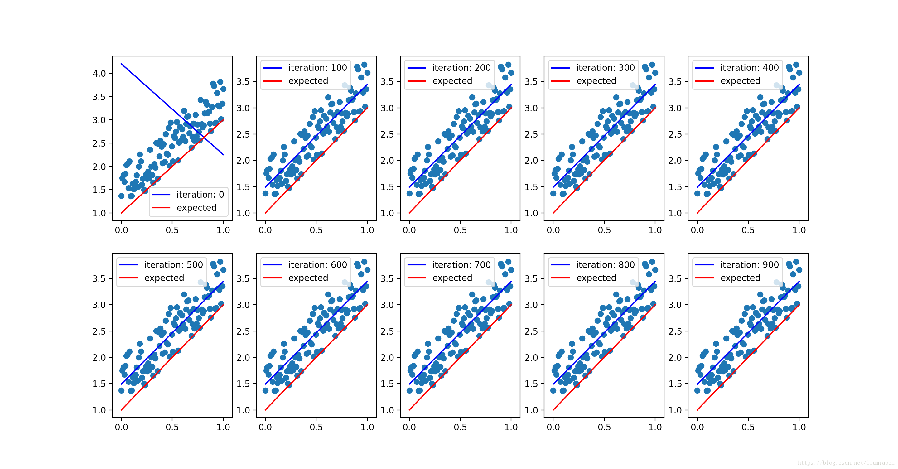
1000次迭代之后的，线性模型如下：

##After Caculation: 
   B: 1.4922265, W : 1.9499784

经过10倍的学习，可以看到逼近没有得到更好的一个效果，结合数据进行确认，发现生成的随机数据和实际的数据已经有了一个偏差，这种情况下只需要进行简单的纠偏即可得到更好的一个结果。

最后

以上就是矮小口红为你收集整理的TensorFlow入门教程：16：随机噪声下的线性回归事前准备示例代码结果确认的全部内容，希望文章能够帮你解决TensorFlow入门教程：16：随机噪声下的线性回归事前准备示例代码结果确认所遇到的程序开发问题。

如果觉得靠谱客网站的内容还不错，欢迎将靠谱客网站推荐给程序员好友。