RNN、LSTM、GRU 的梯度消失及梯度爆炸

RNN

RNN 结构

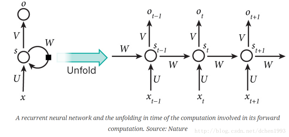
RNN 所有的隐层共享参数 $(U,V,W)$。

前向传播

假设 $t$ 时刻的输入为 $x_t$， 隐藏状态为 $s_t$，输出为 $o_t$，那么
$$s_t=f(W{s}_{t-1}+U{x}_t)$$$$o_t=g(V{s}_t)$$
其中，$f,g$ 为激活函数，$f$ 常取 $tanh$，$g$ 用于预测，常取 $softmax$。

损失函数

假设用于序列建模，输入为 $(x_1,x_2,...,x_T)$ ，标签为 $(y_1,y_2,...,y_T)$，模型的输出为 $(o_1,o_2,...,o_T)$。那么该样本的损失一般可写为 ：
$$L=\sum _{t=1}^T{L}_t$$$$L_t=loss\_function(y_t,o_t)$$

后向传播（BPTT）

RNN 使用梯度下降更新参数 $(W,V,U)$。参数 $V$ 的更新较为简单:
$$\frac{\partial L}{\partial V}=\sum _{t=1}^T\frac{\partial L_t}{\partial V}=\sum _{t=1}^T\frac{\partial L_t}{\partial o_t}\frac{\partial o_t}{\partial V}$$

其中，$\frac{\partial L_t}{\partial o_t}$ 可以根据损失函数的形式以及 $L_t,o_t，y_t$ 的值进行计算，$\frac{\partial o_t}{\partial V}$ 可以根据激活函数 $g$ 的形式以及 $o_t,s_t,V$的值进行计算。

对于参数 $W,U$，$s_t$ 是 $W,U$ 的函数，$s_t=f(W{s}_{t-1}+U{x}_t)$。但是RNN所有隐层共享参数，在这个函数中，$s_{t-1}$ 也是 $W,U$ 的函数。

对于参数 $W$ （$U$ 同理） :
$$\frac{\partial L}{\partial W}=\sum _{t=1}^T\frac{\partial L_t}{\partial W}=\sum _{t=1}^T\frac{\partial L_t}{\partial o_t}\frac{\partial o_t}{\partial s_t}\frac{\partial s_t}{\partial W}$$

根据链式法则:
$$\frac{\partial s_t}{\partial W}=[\frac{\partial s_t}{\partial W}{]}^{+}+\frac{\partial s_t}{\partial s_{t-1}}\frac{\partial s_{t-1}}{\partial W}$$
其中，$[\frac{\partial s_t}{\partial W}{]}^{+}$ 表示 $s_t$ 不考虑 $s_{t-1}$ 时直接对 $W$ 求导。而对于 $\frac{\partial s_{t-1}}{\partial W}$，同理：
$$\frac{\partial s_{t-1}}{\partial W}=[\frac{\partial s_{t-1}}{\partial W}{]}^{+}+\frac{\partial s_{t-1}}{\partial s_{t-2}}\frac{\partial s_{t-2}}{\partial W}$$$$\frac{\partial s_t}{\partial W}=[\frac{\partial s_t}{\partial W}{]}^{+}+\frac{\partial s_t}{\partial s_{t-1}}\frac{\partial s_{t-1}}{\partial W}=[\frac{\partial s_t}{\partial W}{]}^{+}+\frac{\partial s_t}{\partial s_{t-1}}([\frac{\partial s_{t-1}}{\partial W}{]}^{+}+\frac{\partial s_{t-1}}{\partial s_{t-2}}\frac{\partial s_{t-2}}{\partial W})$$$$=[\frac{\partial s_{t-1}}{\partial W}{]}^{+}+\frac{\partial s_t}{\partial s_{t-1}}[\frac{\partial s_{t-1}}{\partial W}{]}^{+}+\frac{\partial s_t}{\partial s_{t-1}}\frac{\partial s_{t-1}}{\partial s_{t-2}}\frac{\partial s_{t-2}}{\partial W}$$
依次对 $s_{t-2},s_{t-3},...,s_1$，最终可得到:
$$\frac{\partial s_t}{\partial W}=\sum _{k=1}^t(\prod _{j=k+1}^t\frac{\partial s_j}{\partial s_{j-1}})[\frac{\partial s_k}{\partial W}{]}^{+}$$
因此:
$$\frac{\partial L}{\partial W}=\sum _{t=1}^T\frac{\partial L_t}{\partial W}$$$$\frac{\partial L_t}{\partial W}=\frac{\partial L_t}{\partial o_t}\frac{\partial o_t}{\partial s_t}\frac{\partial s_t}{\partial W}=\frac{\partial L_t}{\partial o_t}\frac{\partial o_t}{\partial s_t}\sum _{k=1}^t(\prod _{j=k+1}^t\frac{\partial s_j}{\partial s_{j-1}})[\frac{\partial s_k}{\partial W}{]}^{+}=\sum _{k=1}^t\frac{\partial L_t}{\partial o_t}\frac{\partial o_t}{\partial s_t}(\prod _{j=k+1}^t\frac{\partial s_j}{\partial s_{j-1}})[\frac{\partial s_k}{\partial W}{]}^{+}$$

当激活函数 $f$ 为 $tanh$ 时：
$$\frac{\partial \tanh x}{\partial x}=1-(\tanh x{)}^2$$$$\prod _{j=k+1}^t\frac{\partial s_j}{\partial s_{j-1}}=\prod _{j=k+1}^t(1-s_j^2)W$$

$(1-s_j^2)\le 1$。当 $W$ 比较小时，而连乘项比较多时，${\prod }_{j=k+1}^t(1-s_j^2)W$ 就会趋近于0。当 $W$ 比较大，${\prod }_{j=k+1}^t(1-s_j^2)W$ 就会趋近于无穷。这就是RNN容易发生梯度消失或梯度爆炸的原因。

• 梯度爆炸直接导致浮点数溢出，因此比较容易观测到。
• 梯度消失则是靠前的输入无法起到作用，因此模型只能“短期记忆”，影响模型的拟合能力与收敛速度，比较难以观察。

此处存疑：$s_j$ 正相关于 $W$，当 $W$ 越大，$s_j$ 越接近于1， $(1-s_j^2)$ 越接近于0，因此 $(1-s_j^2)W$ 未必会越大而产生梯度爆炸（欢迎探讨）。相对而言，梯度消失更容易发生。只要 $W$ 小于1，且序列足够长，就会发生梯度消失。RNN的梯度消失和深层神经网络的梯度消失不同，深层神经网络的梯度消失一般指层数过深，前面的层因为梯度回传（每一层的梯度不一样）相乘次数多的结果趋近于0，RNN的梯度消失并非指总的梯度趋近于0，而是指参数的更新受近距离的梯度主导（近距离的梯度不会消失），很难学到远距离的关系（远距离的梯度会消失）。

由此可以看出，梯度爆炸或者梯度消失主要是因为BPTT时梯度过大或者梯度过小而导致的，那么可以采取以下方法进行改善:

• 梯度截断（gradient clipping)。设置一个阈值，使梯度不超过这个阈值，当梯度超过时使用阈值代替或对梯度进行放缩。
• 使用非饱和激活函数，如ReLU及其变体。sigmoid 和 tanh 作为激活函数时会将实值放缩到小于1的区域内，从而更容易发生梯度消失。

ReLU不会对原来的梯度进行放缩，因此很难发生梯度消失。某次梯度比较大，参数更新完小于0，那么ReLU梯度就会变成0，不会发生梯度消失，但是该参数会死掉，即永远不会更新， Leaky ReLU 等变体可改善该问题。

LSTM

LSTM 结构

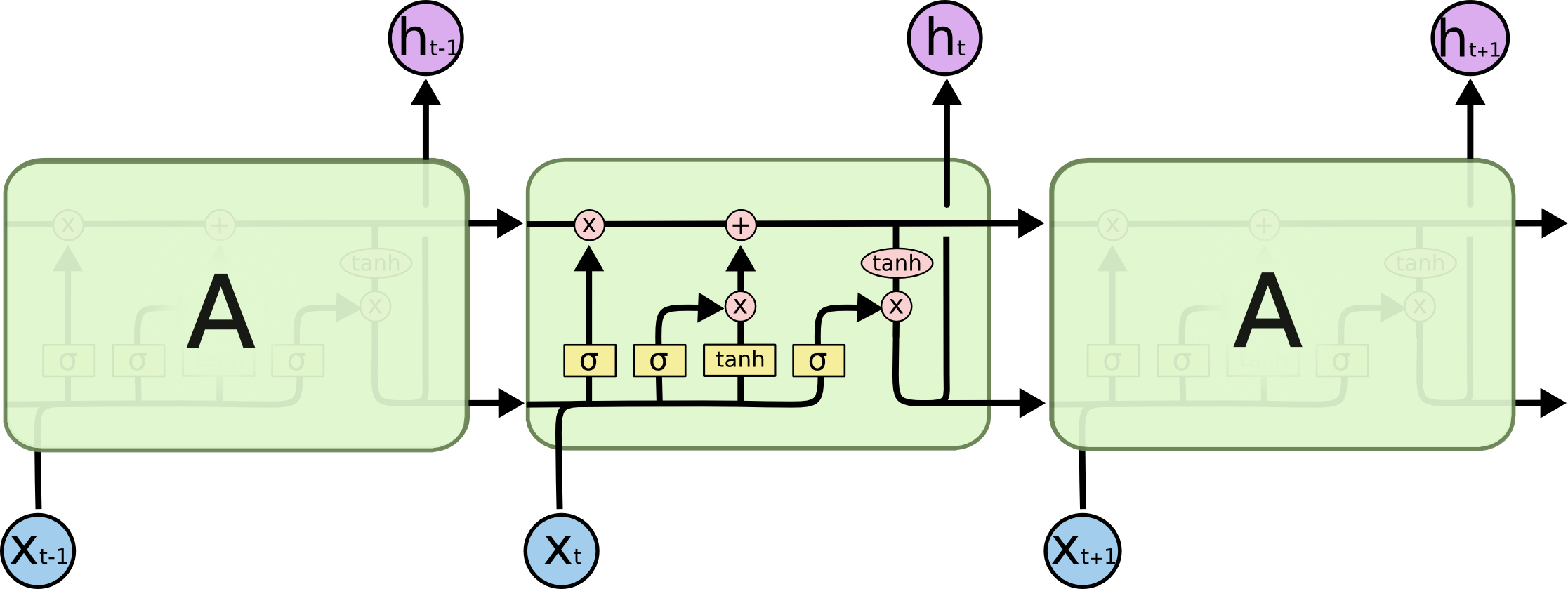
LSTM 主要有三个门结构：输入门、遗忘门、输出门。

前向传播

遗忘门：
$$f_t=sigmoid(W_f[h_{t-1},x_t]+b_f)$$
输入门：
$$i_t=sigmoid(W_i[h_{t-1},x_t]+b_i)$$$${\hat{C}}_t=tanh(W_c[h_{t-1},x_t]+b_c)$$
更新记忆：
$$C_t=f_t\ast C_{t-1}+i_t\ast {\hat{C}}_t$$
输出门：
$$o_t=sigmoid(W_o[h_{t-1},x_t]+b_o)$$$$h_t=o_t\ast tanh(C_t)$$
其中，$\ast$ 表示矩阵对应元素相乘。

后向传播

LSTM的计算较为复杂，后向传播求导非常麻烦。因此这里只理解LSTM为何能够缓解RNN存在的梯度消失/梯度爆炸。LSTM中实际上有两个记忆单元，$C_t$ 和 $h_t$，考虑 $C_t$：
$$C_t=f_t\ast C_{t-1}+i_t\ast {\hat{C}}_t$$
考虑 $C_t$ 中的第 $i$ 个元素：
$$C_{t,i}=f_{t,i}{C}_{t-1,i}+i_{t,i}{\hat{C}}_{t,i}$$
那么：
$$\frac{\partial C_{t,i}}{\partial C_{t-1,i}}=f_{t,i}+\frac{\partial f_{t,i}}{\partial C_{t-1,i}}+\frac{\partial i_{t,i}{\hat{C}}_{t,i}}{\partial C_{t-1,i}}$$

RNN的梯度下降是单项式连乘，LSTM则是多项式相乘，其次LSTM的梯度向后传播过程有非常多的路径，上述过程只是其中的一种，只用了对应元素相乘和相加，更为稳定，因此LSTM更难发生梯度消失。但是，总路径没有梯度消失不代表所有路径都没有梯度消失，某些路径后向传播时仍然是发生了梯度消失的。

早期的LSTM实际上是没有遗忘门的，即相当于 $f_{t,i}=1$，因此连乘不会导致梯度消失。在添加遗忘门后，如果遗忘门接近 1（如模型初始化时会把 $b_f$ 设置成较大的正数，让遗忘门饱和），远距离的梯度不会消失；如果遗忘门接近 0，更有可能是模型学到了某些特征（如文本中的 “not”、“but” 等）选择对前面数据进行遗忘。大多数情况下遗忘门仍然是一个0~1的数，LSTM 仍然是有可能发生梯度消失的，只是概率远远低于RNN。

LSTM 仍然是有可能发生梯度爆炸的，但是因为回传路径复杂多样，并且可能经过多个激活函数，因此频率比较低。实际中梯度爆炸一般结合梯度裁剪 (gradient clipping) 解决。

梯度仅仅是LSTM的有效性的一个方面，LSTM的有效性可以从多视角理解，如建模、信息选择上。如 Written Memories: Understanding, Deriving and Extending the LSTM。

GRU

GRU 结构

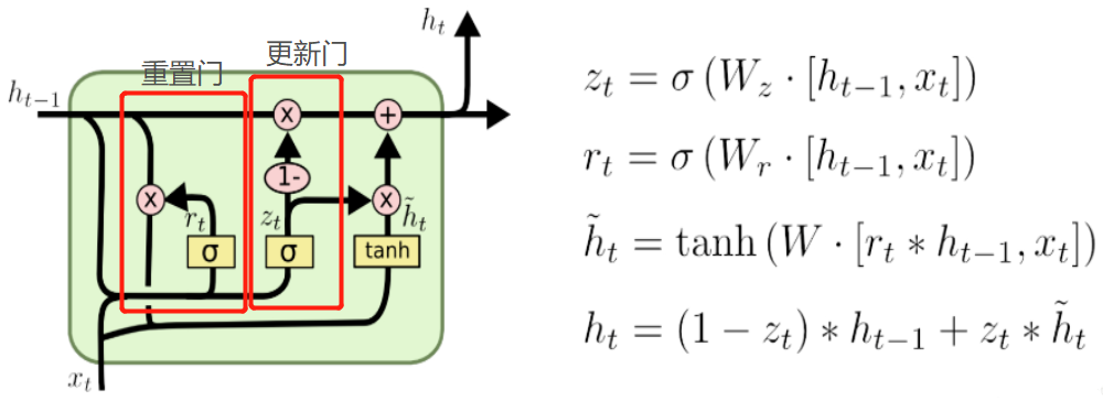
GRU分为重置门和更新门：

前向传播

重置门：
$$z_t=sigmoid(W_z[h_{t-1},x_t])$$
更新门：
$$r_t=sigmoid(W_r[h_{t-1},x_t])$$$${\hat{h}}_t=tanh(W[r_t\ast h_{t-1},x_t])$$
更新记忆状态:
$$h_t=(1-z_t)\ast h_{t-1}+z_t\ast {\hat{h}}_t$$

后向传播

关于梯度消失和梯度爆炸的分析类似于LSTM。GRU相对于LSTM参数更少，训练更快。理论上GRU记忆能力相对弱于LSTM，但是实际上很难判定优劣，一般通过实验进行选择。

Reference

• https://www.zhihu.com/question/34878706
  
• Written Memories: Understanding, Deriving and Extending the LSTM

最后

以上就是深情胡萝卜最近收集整理的关于RNN、LSTM、GRU 的梯度消失及梯度爆炸RNN、LSTM、GRU 的梯度消失及梯度爆炸的全部内容，更多相关RNN、LSTM、GRU内容请搜索靠谱客的其他文章。