信号处理基础-matlab-wavread-audioread

98 阅读 0 评论 65 点赞

我是靠谱客的博主紧张眼睛，这篇文章主要介绍信号处理基础-matlab-wavread-audioread，现在分享给大家，希望可以做个参考。

信号处理基础

实验目的
了解音频和图像数据系数特点，掌握音频和图像文件的离散傅里叶，离散余弦和离散小波变换等基本条件
实验环境
(1）windows10
(2)Matlab2020
(3)bmp格式图像文件
(4）wav格式音频文件
1.用离散傅里叶变换分析合成音频和图像分析合成音频文件包括一下步骤：
（1）读取音频文件数据；

复制代码

1
2
3
4
5
6
7
8
clc;
clear;
len=40000;
[fn,pn]=uigetfile('*.wav','请选择音频文件');
filename=strcat(pn,fn);
[x,fs]=audioread(filename,[1,len]);

注意：新版本的matlab中已经不再支持wavread()函数，替代函数为audioread(filename,N),其中N必须为[m,n]格式，如[2,100],且m,n均为正数
进行一维离散傅里叶变换：（其中fft()函数为一维离散傅里叶变换函数，fftshift函数将零频对应系数移至中央）

复制代码

1
2
3
4
5
6
xf=fft(x);
f1=[0:len-1]*fs/len;
xff=fftshift(xf);
h1=floor(len/2);
f2=[-h1:h1]*fs/len;

进行一维离散傅里叶逆变换：

复制代码

1
2
xsync=ifft(xf);

显示图像代码：

复制代码

1
2
3
4
5
6
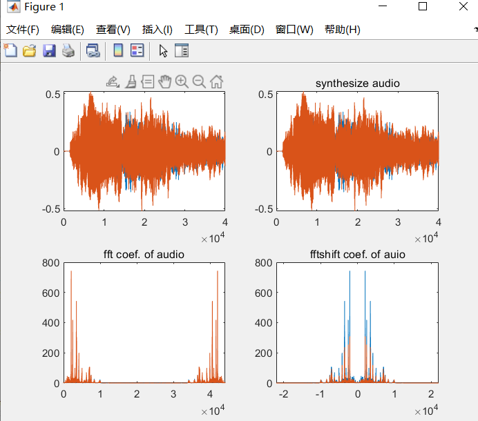
figure;
subplot(2,2,1);plot(x);title('original audio');
subplot(2,2,2);plot(xsync);title('synthesize audio');
subplot(2,2,3);plot(f1,abs(xf));title('fft coef. of audio');
subplot(2,2,4);plot(f2(1:len),abs(xff));title('fftshift coef. of auio');

结果：
在这里插入图片描述

（2）分析合成图像文件：

读取图像文件数据：

复制代码

1
2
3
4
[fn,pn]=uigetfile('*.bmp','请选择图像文件');
[x,map]=imread(strcat(pn,fn),'bmp');
I=rgb2gray(x);

二维离散傅里叶变换：

复制代码

1
2
3
xf=fft2(I);
xff=fftshift(xf);

二维离散傅里叶逆变换：

复制代码

1
2
xsync=ifft2(xf);

观察结果：

复制代码

1
2
3
4
5
6
figure;
subplot(2,2,1);imshow(x);title('original image');
subplot(2,2,2);imshow(uint8(abs(xsync)));title('synthesize image');
subplot(2,2,3);mesh(abs(xf));title('fft coef. of image');
subplot(2,2,4);mesh(abs(xff));title('fftshift coef. of image');

结果：
在这里插入图片描述

2.用离散余弦变换分析合成音频和图像

（1）分析合成音频文件数据：
读取音频文件数据：

复制代码

1
2
3
4
5
6
7
clc;
clear;
len=40000;
[fn,pn]=uigetfile('*.wav','请选择音频文件');
filename=strcat(pn,fn);
[x,fs]=audioread(filename,[1,len]);

一维离散余弦变换：

复制代码

1
2
xf=dct(x);

一维离散余弦逆变换：

复制代码

1
2
3
4
5
6
xsync=idct(xf);
[row,col]=size(x);
xff=zeros(row,col);
xff(1:row,1:col)=xf(1:row,1:col);
y=idct(xff);

观察结果：

复制代码

1
2
3
4
5
6
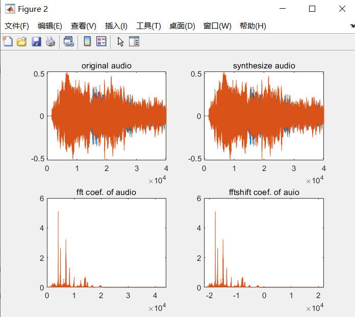
figure;
subplot(2,2,1);plot(x);title('original audio');
subplot(2,2,2);plot(xsync);title('synthesize audio');
subplot(2,2,3);plot(f1,abs(xf));title('fft coef. of audio');
subplot(2,2,4);plot(f2(1:len),abs(xff));title('fftshift coef. of auio');

需要注意的是，上述代码中用到的f1,f2在前文的代码中

复制代码

1
2
3
f1=[0:len-1]*fs/len;
f2=[-h1:h1]*fs/len;

结果显示：
在这里插入图片描述

（2）分析合成图像文件数据：
读取图像文件数据：

复制代码

1
2
3
4
[fn,pn]=uigetfile('*.bmp','请选择图像文件');
[x,map]=imread(strcat(pn,fn),'bmp');
I=rgb2gray(x);

二维离散余弦变换：

复制代码

1
2
xf=dct2(I);

二维离散余弦逆变换：

复制代码

1
2
3
4
5
6
7
8
9
xsync=uint8(idct(xf));
[row,col]=size(I);
lenr=round(row*4/5);
lenc=round(col*4/5);
xff=zeros(row,col);
xff=zeros(row,col);
xff(1:lenr,1:lenc)=xf(1:lenr,1:lenc);
y=uint8(idct2(xff));

观察结果：

复制代码

1
2
3
4
5
6
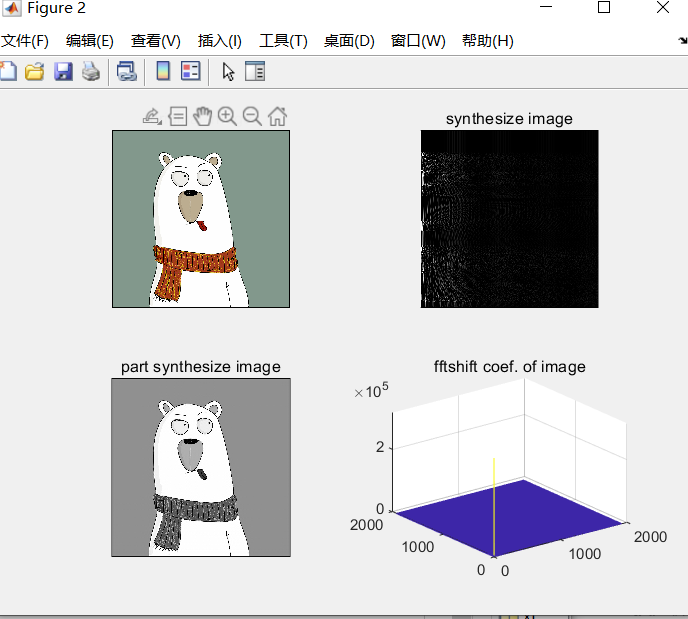
figure;
subplot(2,2,1);imshow(x);title('original image');
subplot(2,2,2);imshow(uint8(abs(xsync)));title('synthesize image');
subplot(2,2,3);imshow(uint8(abs(y)));title('part synthesize image');
subplot(2,2,4);mesh(abs(xff));title('fftshift coef. of image');

结果显示：
在这里插入图片描述

3.用离散小波变换分析合成音频和图像
（1）分析合成音频文件包括以下步骤：
读取音频文件数据：

复制代码

1
2
3
4
5
6
7
clc;
clear;
len=40000;
[fn,pn]=uigetfile('*.wav','请选择音频文件');
filename=strcat(pn,fn);
[x,fs]=audioread(filename,[1,len]);

如果你的音乐文件是多声道的还需要加上下面的代码，将多声道转换为单声道

复制代码

1
2
x=x(:,1);

一维离散小波变换：

复制代码

1
2
[C,L]=wavedec(x,2,'db4');

一维离散小波逆变换：

复制代码

1
2
3
4
5
6
xsync=waverec(C,L,'db4');
cA2=appcoef(C,L,'db4',2);
cD2=detcoef(C,L,2);
cD1=detcoef(C,L,1);

观察结果：

复制代码

1
2
3
4
5
6
7
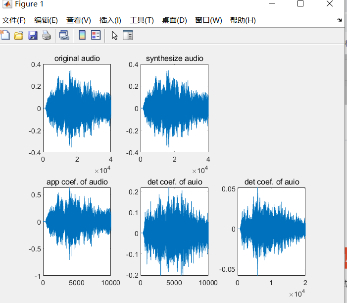
figure;
subplot(2,3,1);plot(x);title('original audio');
subplot(2,3,2);plot(xsync);title('synthesize audio');
subplot(2,3,4);plot(cA2);title('app coef. of audio');
subplot(2,3,5);plot(cD2);title('det coef. of auio');
subplot(2,3,6);plot(cD1);title('det coef. of auio');

结果显示：
在这里插入图片描述

（2）分析合成图像文件包括以下步骤：
读取图像文件数据：

复制代码

1
2
3
4
[fn,pn]=uigetfile('*.bmp','请选择图像文件');
[x,map]=imread(strcat(pn,fn),'bmp');
I=rgb2gray(x);

二维离散小波变换：

复制代码

1
2
3
sx=size(I);
[cA1,cH1,cV1,cD1]=dwt2(I,'bior3.7');

二维离散小波逆变换：

复制代码

1
2
3
4
5
6
7
xsync=uint8(idwt2(cA1,cH1,cV1,cD1,'bior3.7',sx));
A1=uint8(idwt2(cA1,[],[],[],'bior3.7',sx));
H1=uint8(idwt2([],cH1,[],[],'bior3.7',sx));
V1=uint8(idwt2([],[],cV1,[],'bior3.7',sx));
D1=uint8(idwt2([],[],[],cD1,'bior3.7',sx));

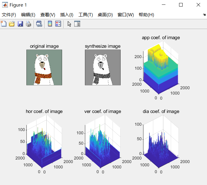
观察结果：

复制代码

1
2
3
4
5
6
7
8
figure;
subplot(2,3,1);imshow(x);title('original image');
subplot(2,3,2);imshow(uint8(abs(xsync)));title('synthesize image');
subplot(2,3,3);mesh(A1);title('app coef. of image');
subplot(2,3,4);mesh(H1);title('hor coef. of image');
subplot(2,3,5);mesh(V1);title('ver coef. of image');
subplot(2,3,6);mesh(D1);title('dia coef. of image');

结果显示：
在这里插入图片描述