NonLinear Regression Problem & Ridge RegressionPart One : Basis for Nonlinear RegressionPart Two : Create a NonLinear Regression problemPart Three : Ridge RegressionPart Four : Visualize the Result

Part One : Basis for Nonlinear Regression

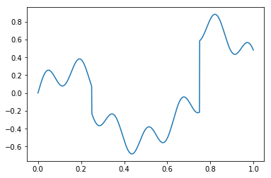
In this part we’re going to investigate how to use linear regression to approximate and estimate complicated functions. For example, suppose we want to fit the following function on the interval [0,1] :

Import Modules

import numpy as np
import matplotlib.pyplot as plt
import pandas as pd

Create a problem

def y(x):
    ret = .15*np.sin(40*x) 
    ret = ret + .25*np.sin(10*x)
    step_fn1 = np.zeros(len(x))
    step_fn1[x >= .25] = 1
    step_fn2 = np.zeros(len(x))
    step_fn2[x >= .75] = 1
    ret = ret - 0.3*step_fn1 + 0.8 *step_fn2 
    return ret

x = np.arange(0.0, 1.0, 0.001)
plt.plot(x, y(x))
plt.show()

Plot the graph and see the functions

Here the input space, shown on the x-axis, is very simple – it’s just the interval $[0,1]$. The output space is reals ($\mathcal{R}$), and a graph of the function { ( x , y ( x ) ) ∣ x ∈ [ 0 , 1 ] } {(x,y(x)) mid x in [0,1]} { (x,y(x))∣x∈[0,1]} is shown above. Clearly a linear function of the input will not give a good approximation to the function. There are many ways to construct nonlinear functions of the input. Some popular approaches in machine learning are regression trees, neural networks, and local regression (e.g. LOESS). However, our approach here will be to map the input space $[0,1]$ into a “feature space” ${\mathcal{R}}^d$, and then run standard linear regression in the feature space.

Feature extraction, or “featurization”, maps an input from some input space $\mathcal{X}$ to a vector in ${\mathcal{R}}^d$. Here our input space is $\mathcal{X}=[0,1]$, so we could write our feature mapping as a function $\Phi :[0,1]\to {\mathcal{R}}^d$. The vector $\Phi (x)$ is called a feature vector, and each entry of the vector is called a feature. Our feature mapping is typically defined in terms of a set of functions, each computing a single entry of the feature vector. For example, let’s define a feature function ${\varphi }_1(x)=1(x\ge 0.25)$. The $1(\cdot )$ denotes an indicator function, which is 1 if the expression in the parenthesis is true, and 0 otherwise. So ${\varphi }_1(x)$ is $1$ if $x\ge 0.25$ and $0$ otherwise. This function produces a “feature” of x. Let’s define two more features: ${\varphi }_2(x)=1(x\ge 0.5)$ and ${\varphi }_3(x)=1(x\ge 0.75)$. Now we can define a feature mapping into ${\mathcal{R}}^3$ as:
$$\Phi (x)=({\varphi }_1(x),{\varphi }_2(x),\varphi$$

最后

以上就是饱满帅哥为你收集整理的NonLinear Regression Problem & Ridge RegressionPart One : Basis for Nonlinear RegressionPart Two : Create a NonLinear Regression problemPart Three : Ridge RegressionPart Four : Visualize the Result的全部内容，希望文章能够帮你解决NonLinear Regression Problem & Ridge RegressionPart One : Basis for Nonlinear RegressionPart Two : Create a NonLinear Regression problemPart Three : Ridge RegressionPart Four : Visualize the Result所遇到的程序开发问题。

如果觉得靠谱客网站的内容还不错，欢迎将靠谱客网站推荐给程序员好友。