机器学习项目实战-能源利用率3-分析

接上一篇: [[ 机器学习项目实战-能源利用率2-建模 ]]

* 导入建模数据

import warning
warning.filterwarning('ignore')

import pandas as pd
import numpy as np
pd.options.mode.chained_assignment = None
pd.set_option('display.max_columns', 50)

import matplotlib.pyplot as plt
import seaborn as sns
%matplotlib inline
plt.rcParams['font.size'] = 24
sns.set(font_scale = 2)

train_features = pd.read_csv('data/training_features.csv')
test_features = pd.read_csv('data/testing_features.csv')
train_labels = pd.read_csv('data/training_labels.csv')
test_labels = pd.read_csv('data/testing_labels.csv')

from sklearn.importer import SimpleImputer
imputer = SimpleImputer(strategy = 'median')
imputer.fit(train_features)
X = imputer.transform(train_features)
X_test = imputer.transform(test_features)

from sklearn.preprocessing import MinMaxScaler
minmax_scaler = MinMaxScaler().fit(X)
X = minmax_scaler.transform(X)
X_test = minmax_scaler.transform(X_test)

y = np.array(train_labels).reshape((-1, ))
y_test = np.array(test_labels).reshape((-1, ))

def mae(y_true, y_pred):
	return np.mean(abs(y_true - y_pred))

from sklearn.ensemble import GradientBoostingRegressor

model = GradientBoostingRegressor(loss = 'lad', max_depth = 6, max_features = None,
                                 min_samples_leaf = 4, min_samples_split = 10, e_estimators = 550, random_state = 42)
model.fit(X, y)

model_pred = model.predict(X_test)
model_mae = mae(y_test, model_pred)
print('Final Model Performance on the test set: MAE = %.4f' % model_mae)

Final Model Performance on the test set: MAE = 9.0963

七. 解释模型

1. 特征重要性
2. Locally Interpretable Model-agnostic Explainer (LIME)
3. 建立一颗树模

7.1 特征重要性

sklearn中特征重要性的计算方法

在所有树模型中平均节点不纯度的减少

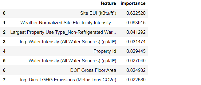
7.1.1 特征重要性排序

feature_results = pd.DataFrame({'feature': list(train_features.columns),
                               'importance': model.feature_importances_})
feature_results = feature_results.sort_values('importance', ascending = False).reset_index(drop = True)
feature_results.head(8)

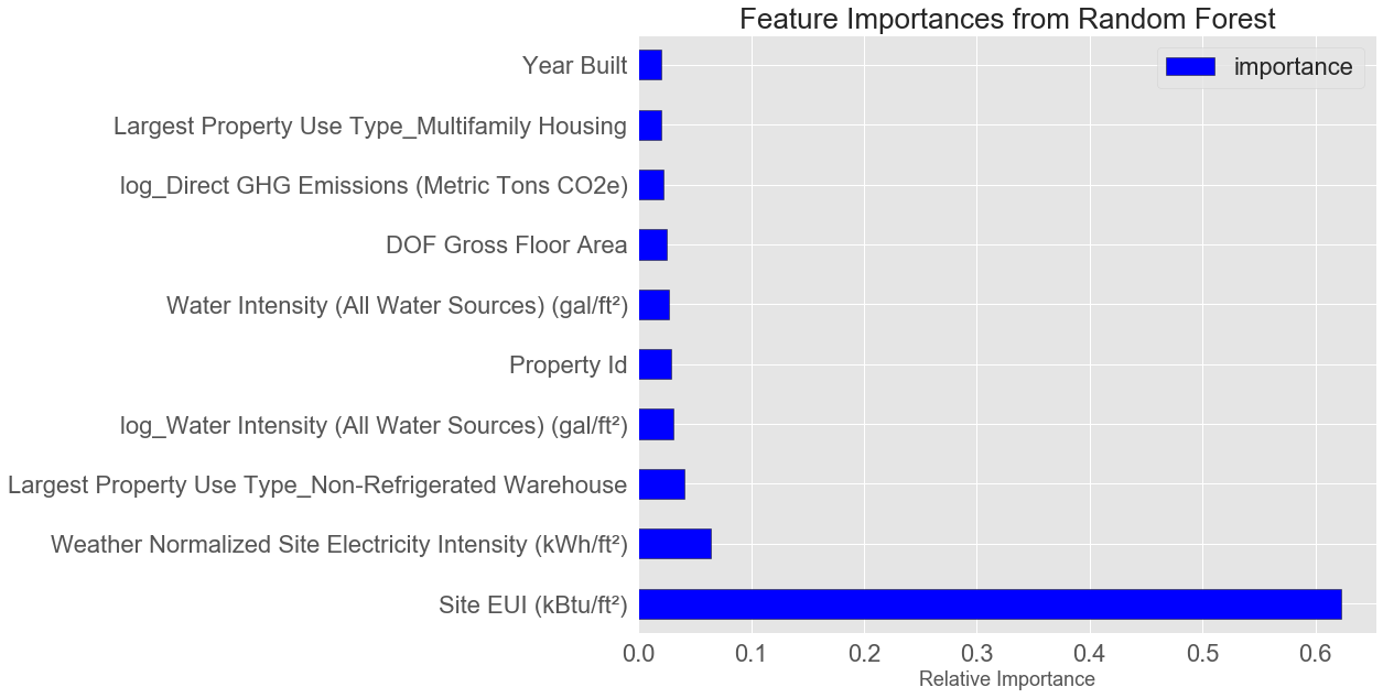
from IPython.core.pylabtools import figsize
figsize(12, 10)
plt.style.use('ggplot')

feature_results.loc[:9, :].plot(x = 'feature', y = 'importance', edgecolor = 'k',
                               kind = 'barh', color = 'blue')
plt.xlabel('Relative Importance', fontsize = 18); plt.ylabel('')
# plt.yticks(fontsize = 12); plt.xticks(fontsize = 14)
plt.title('Feature Importances from Random Forest', size = 26)

7.1.2 特征重要性95%

cumulative_importances = np.cumsum(feature_results['importance'])

plt.figure(figsize = (20, 6))
plt.plot(list(range(feature_results.shape[0])), cumulative_importances.values, 'b-')
plt.hlines(y=0.95, xmin=0, xmax=feature_results.shape[0], color='r', linestyles='dashed')
# plt.xticks(list(range(feature_results.shape[0])), feature_results.feature, rotation=60)
plt.xlabel('Feature', fontsize = 18)
plt.ylabel('Cumulative importance', fontsize = 18)
plt.title('Cumulative Importances', fontsize = 26)

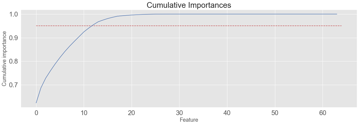
most_num_importances = np.where(cumulative_importances > 0.95)[0][0] + 1
print('Number of features for 95% importance: ', most_num_importances)

Number of features for 95% importance: 13

7.1.3 根据特征重要性筛选特征

most_important_features = feature_results['feature'][:13]
indices = [list(train_features.columns).index(x) for x in most_important_features]
X_reduced = X[:, indices]
X_test_reduced = X_test[:, indices]

pirnt('Most import training features shape: ', X_reduced.shape)
print('Most import testing feature shape: ', X_test_reduced.shape)

Most import training features shape: (6622, 13)
Most import testing features shape: (2839, 13)

7.1.4 检测效果

from sklearn.ensemble import RandomForestRegressor
rfr = RandomForestRegressor(random_state = 42)

rfr.fit(X, y)
rfr_full_pred = rfr.predict(X_test)

rfr.fit(X_reduced, y)
rfr_reduced_pred = rfr.predict(X_test_reduced)

print('Random Forest Full Results: MAE =    %.4f.' % mae(y_test, rfr_full_pred))
print('Random Forest Reduced Results: MAE = %.4f.' % mae(y_test, rfr_reduced_pred))

from sklearn.linear_model import LinearRegression
lr = LinearRegression()

lr.fit(X, y)
lr_full_pred = lr.predict(X_test)

lr.fit(X_reduced, y)
lr_reduced_pred = lr.predict(X_test_reduced)

print('Linear Regression Full Results: MAE =    %.4f.' % mae(y_test, lr_full_pred))
print('Linear Regression Reduced Results: MAE = %.4f.' % mae(y_test, lr_reduced_pred))

Random Forest Full Results: MAE = 9.9025.
Random Forest Reduced Results: MAE = 10.3780.
Linear Regression Full Results: MAE = 13.4651.
Linear Regression Reduced Results: MAE = 14.3103.

• 试验结果发现效果还不如原来

model_reduced = GradientBoostingRegressor(loss = 'lad', max_depth = 6, max_features = None,
                                 min_samples_leaf = 4, min_samples_split = 10,
                                 n_estimators = 550, random_state = 42)
model_reduced.fit(X_reduced, y)
model_reduced_pred = model_reduced.predict(X_test_reduced)

print('Gradient Boosting Reduced Results: MAE = %.4f.' % mae(y_test, model_reduced_pred))

Gradient Boosting Reduced Results: MAE = 9.3899.

• 在GBDT中出现了同样的问题，所以不选择去掉部分小价值特征。

7.2 LIME

Locally Interpretable Model-agnostic Explanations
地址：LIME to explain individual predictions
分别选择一个预测最好的和预测最差的来分别解释

7.2.1 最差预测的解释

import lime
import lime.lime_tabular

residuals = abs(model_reduced_pred - y_test) # 残差
wrong = X_test_reduced[np.argmax(residuals), :] # 最差的预测
right = X_test_reduced[np.argmin(residuals), :] # 最好的预测

# 最差预测位置的预测值与真实值
print('Prediction: %.4f' % model_reduced.predict(wrong.reshape(1, -1)))
print('Actual Value: %.4f' % y_test[np.argmax(residuals)])

# Create a lime explainer object
explainer = lime.lime_tabular.LimeTabularExplainer(training_data = X_reduced, mode = 'regression',
            training_labels = y, feature_names = list(most_important_features))

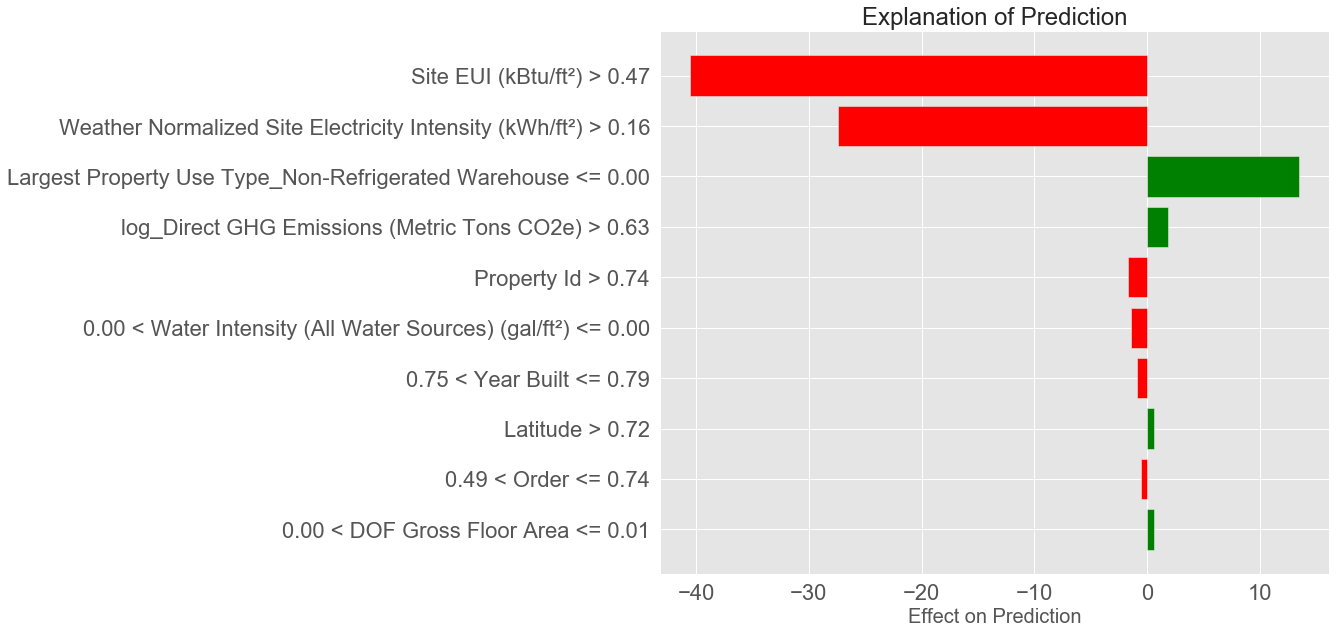
# 最差预测的解释
wrong_exp = explainer.explain_instance(data_row = wrong, predict_fn = model_reduced.predict)

# 预测的解释画图
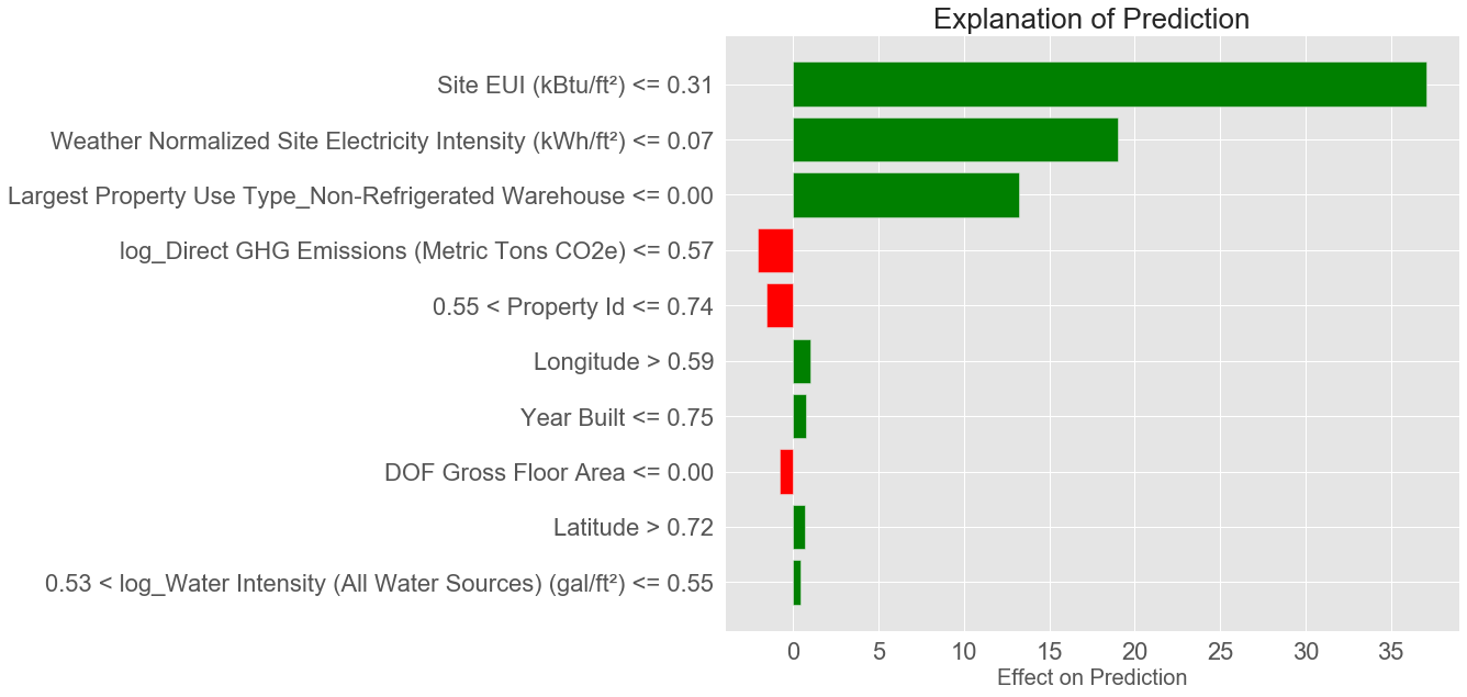
wrong_exp.as_pyplot_figure()
plt.title('Explanation of Prediction', fontsize = 24)
plt.xlabel('Effect on Prediction', fontsize = 20)

Prediction: 11.6612
Actual Value: 96.0000

wrong_exp.show_in_notebook(show_predicted_value = False)

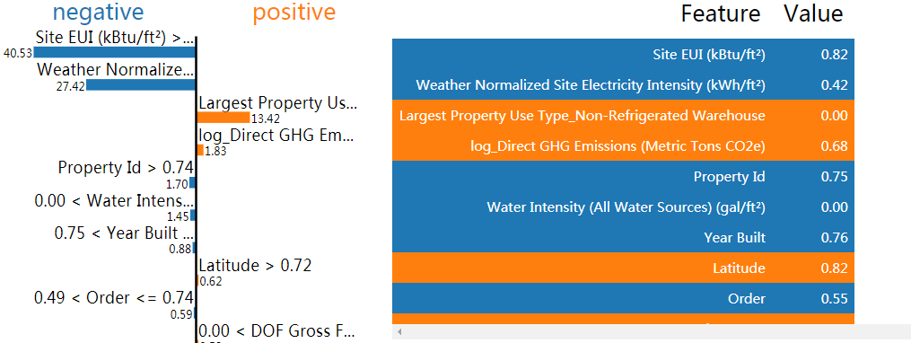
预测值：11.66 实际值：96。这里面差距实在太大了，会不会存在什么问题呢？

上图展示了各个特征对结果的贡献程度，其中Site EUI使得结果值大大下降，由于该值(归一化后) 大于0.47了，正常情况下是能源利用率较低了，但是这里反而标签的得分很高，所以有理由认为，该数据点标签值存在问题。

7.2.2 最好预测的解释

# 最好预测位置的预测值与真实值
print('Prediction: %0.4f' % model_reduced.predict(right.reshape(1, -1)))
print('Actual Value: %0.4f' % y_test[np.argmin(residuals)])

# 最好预测的解释
right_exp = explainer.explain_instance(data_row = right, predict_fn = model_reduced.predict, num_features = 10)

# 预测的解释画图
right_exp.as_pyplot_figure()
plt.title('Explanation of Prediction', size = 26)
plt.xlabel('Effect on Prediction', size = 20)

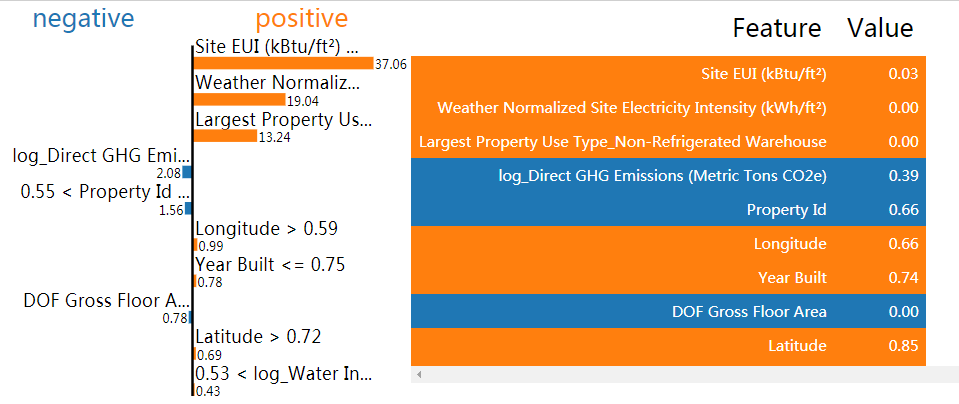
Prediction: 99.9975
Actual Value: 100.0000

right_exp.show_in_notebook(show_predicted_value = False)

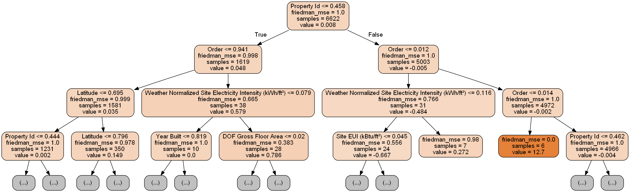
7.3 单棵树模型观察

from sklearn import tree
import pydotplus
from IPython.display import display, Image

single_tree = model_reduced.estimators_[100][0]

dot_data = tree.export_graphviz(single_tree, out_file = None, rounded = True,
                    feature_names = most_important_features, filled = True)
graph = pydotplus.graph_from_dot_data(dot_data)
graph.write_png('sigle_tree.png')
display(Image(graph.creat_png()))

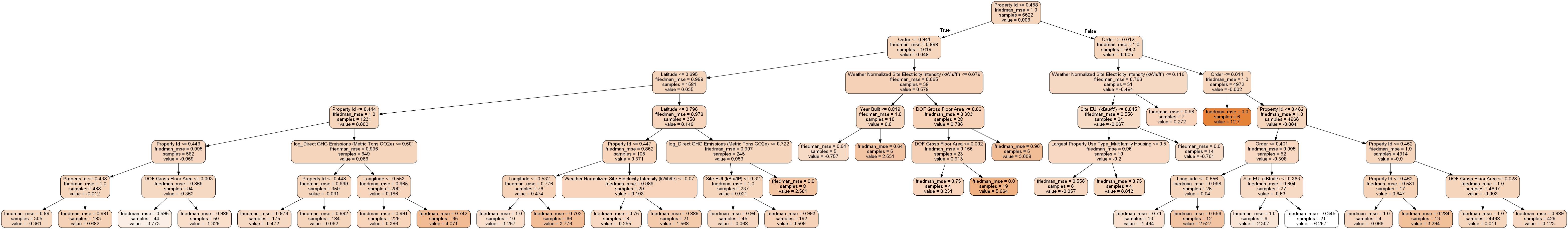
• 太密集了，限制下深度

dot_data = tree.export_graphviz(single_tree, out_file = None, rounded = True,
                    max_depth = 3, feature_names = most_important_features, filled = True)
graph = pydotplus.graph_from_dot_data(dot_data)
graph.write_png('sigle_tree.png')
display(Image(graph.create_png()))

最后

以上就是饱满咖啡豆为你收集整理的机器学习项目实战-能源利用率3-分析的全部内容，希望文章能够帮你解决机器学习项目实战-能源利用率3-分析所遇到的程序开发问题。

如果觉得靠谱客网站的内容还不错，欢迎将靠谱客网站推荐给程序员好友。