本文是 2020人工神经网络第一次作业 的参考答案第四部分
➤04 第四题参考答案
1.使用BP网络逼近Hermit函数
f
(
x
)
=
1.1
(
1
−
x
+
2
x
2
)
⋅
e
−
x
2
2
fleft( x right) = 1.1left( {1 - x + 2x^2 } right) cdot e^{ - {{x^2 } over 2}}
f(x)=1.1(1−x+2x2)⋅e−2x2
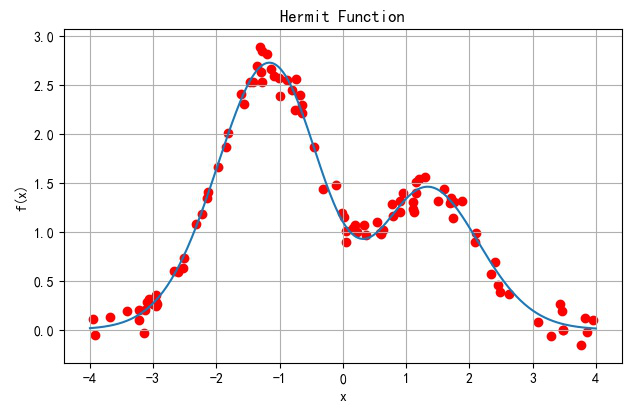
▲ Hermit函数 以及相关函数随机采集数据(红色)
def Hermit(x):
    return 1.1 * (1 - x + 2 * x * x) * exp(-x**2/2)

x = linspace(-4, 4, 250)
fx = Hermit(x)

sx = random.uniform(-4, 4, 100)
fs = Hermit(sx) + random.normal(0, 0.1, len(sx))
(1) 隐层节点:10
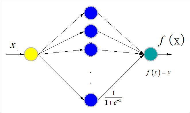
▲ 网络结构
上述BP网络实现程序参见后附录中的:1.BP网络函数逼近程序
训练超参数:
- 学习速率:
η
=
0.5
eta = 0.5
η=0.5
▲ 收敛过程中网络输出输入之间函数变化过程
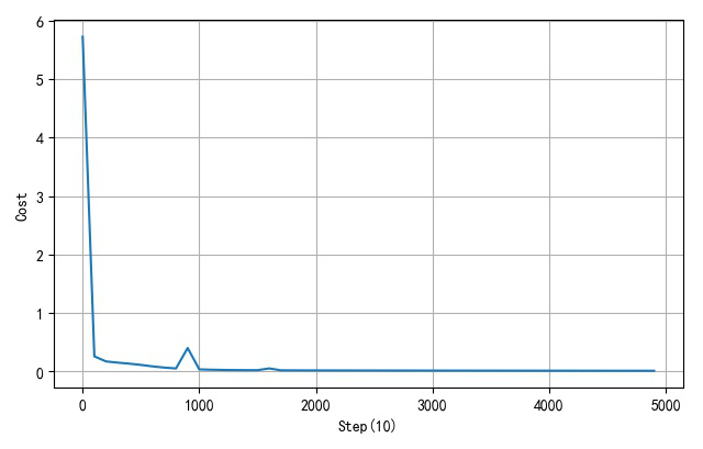
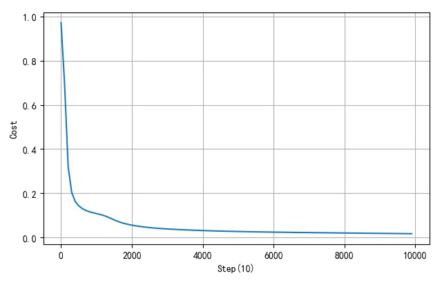
▲ 网络训练误差收敛曲线
(2) 不同隐层节点个数
- 隐层三个节点:
▲ 隐层三个节点训练过程
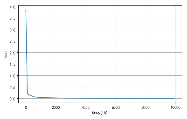
▲ 隐层三个节点网络误差收敛曲线
- 隐层节点数量:20
▲ 隐层20个节点网络训练过程
▲ 隐层20个节点网络误差收敛过程
(3) 不同隐层节点数目与网络误差
构造不同隐层节点数量(2,3,…,10),使用学习速率0.5, 训练10000循环,对应的网络收敛后的不同的误差。
| 隐层节点个数 | 2 | 3 | 4 | 5 | 6 | 7 | 8 | 9 | 10 |
|---|---|---|---|---|---|---|---|---|---|
| 网络逼近误差 | 0.1122 | 0.0202 | 0.00927 | 0.0102 | 0.01016 | 0.00704 | 0.01017 | 0.006515 | 0.009511 |
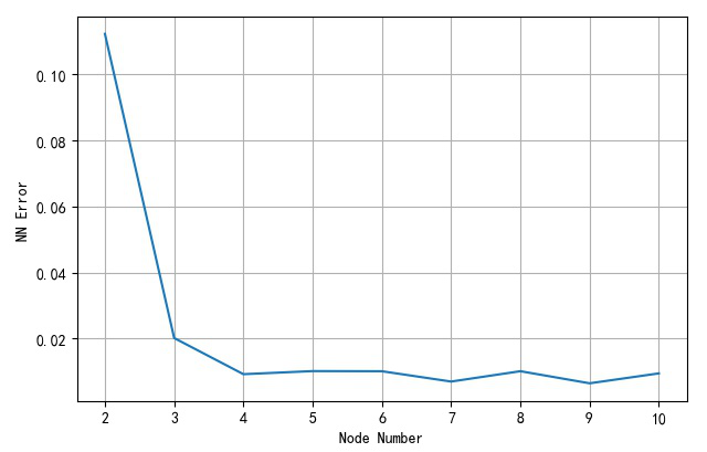
▲ 不同的隐层节点对应网络逼近误差
从上面训练结果可以看到,当隐层节点大于等4之后,网络对于Hermit函数逼近的精度就降低到0.01之下了。
2.使用RBF网络进行函数逼近
(1) 训练样本
样本数取32个。在[-4,4]之间均匀分布,同样添加标准差为0.1的正态分布噪声。下面红色点为加有噪声之后的训练样本。

▲ Hermit函数以及均匀采样的32个样本
def Hermit(x):
    return 1.1 * (1 - x + 2 * x * x) * exp(-x**2/2)

x_line = linspace(-4, 4, 250)
y_line = Hermit(x_line)
x_train = linspace(-4, 4, 30)
y_train = Hermit(x_train) + random.normal(0, 0.1, len(x_train))
(2) 网络结构
构建RBF网络,选择RBF网络隐层节点的个数 N h ∈ ( 3 , 30 ) N_h in left( {3,,,,30} right) Nh∈(3,30)。隐层节点的径向基函数采用高斯函数形式的函数:
f ( x ) = e − ∣ x − x c ∣ 2 2 σ 2 fleft( x right) = e^{ - {{left| {x - x_c } right|^2 } over {2sigma ^2 }}} f(x)=e−2σ2∣x−xc∣2
每个隐层神经元的参数包括:中心 x c x_c xc,方差: σ sigma σ。
RBF网络Python实现程序参见后面附录中的:2.RBF网络实现程序
(3) 网络训练
由于训练样本是在(-4,4)之间的均匀采样,所以构造隐层节点的中心 x c x_c xc位置也在(-4,4)之间均匀采样。隐层节点的方差取隐层节点中心平均距离: σ = 8 N h sigma = {8 over {N_h }} σ=Nh8。
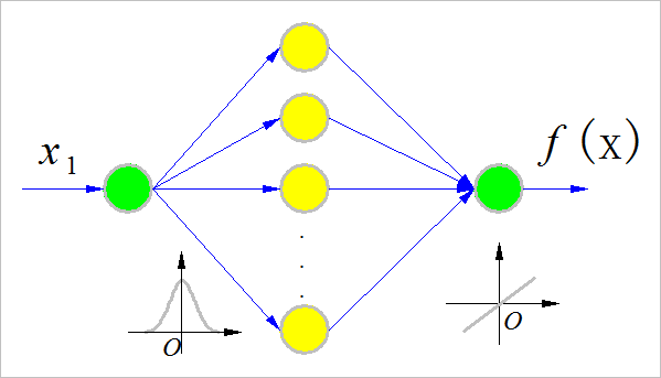
▲ RBF网络结构
在这里,选取网络隐层节点个数: N h = 10 N_h = 10 Nh=10。
隐层各节点的中心位置:
| Node#10 | -4.00 | -3.11 | -2.22 | -1.33 | -0.44 | 0.44 | 1.33 | 2.22 | 3.11 | 4.00 |
|---|
根据训练样本 { x i , y i } i = 1 , ⋯ , 30 left{ {x_i ,y_i } right}_{i = 1, cdots ,30} {xi,yi}i=1,⋯,30,计算出隐层对应的输出矩阵: H 30 = { h 1 , h 2 , ⋯ , h 30 } H_{30} = left{ {h_1 ,h_2 , cdots ,h_{30} } right} H30={h1,h2,⋯,h30},其中每个 h i h_i hi都对应着某一个样本 x i x_i xi输入之后得到的隐层输出。
RBF网络输出为: y ^ i = W T ⋅ h i hat y_i = W^T cdot h_i y^i=WT⋅hi
其中 W W W是隐层到网络试试部分的链接权系数。
将样本的期望输出组成向量: y ˉ = { y 1 , y 2 , ⋯ , y 30 } T bar y = left{ {y_1 ,y_2 , cdots ,y_{30} } right}^T yˉ={y1,y2,⋯,y30}T
对于隐层到输出节点的加权系数 W W W,可以直接通过求取伪逆的方式获得:
W T = y ˉ ⋅ ( H 30 T ⋅ H 30 + λ ⋅ I 30 ) − 1 ⋅ H 30 T W^T = bar y cdot left( {H_{30}^T cdot H_{30} + lambda cdot I_{30} } right)^{ - 1} cdot H_{30}^T WT=yˉ⋅(H30T⋅H30+λ⋅I30)−1⋅H30T
其中 λ ⋅ I 30 lambda cdot I_{30} λ⋅I30加入放置矩阵求逆出现奇异设定的。 λ lambda λ可以选取一个比较小的数值,比如0.0001。
(4) 训练结果
通过上方法得到RBF网络参数:隐层节点的径向基函数的中心点,方差,隐层到输出层的加权系数,RBF网络便设计完成了。
下面是网络构建之后,实际对应的函数关系。对于训练样本数据,网络的误差为: V a r ( [ y ^ i − y i ] i = 1 , 2 , ⋯ , 30 ) = 0.00569 Varleft( {left[ {hat y_i - y_i } right]_{i = 1,2, cdots ,30} } right) = 0.00569 Var([y^i−yi]i=1,2,⋯,30)=0.00569
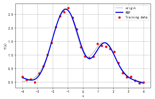
▲ 隐层节点为10 的情况下RBF网络函数拟合的结果
(5) 不同隐层节点对应训练误差
选取网络中间隐层节点的个数 N h N_h Nh从3变化到30,对应网络训练结果如下。
▲ 不同隐层节点数量对应网络结果
随着RBF网络隐层节点个数从3变化到30,对应的网络训练误差的变化曲线如下:
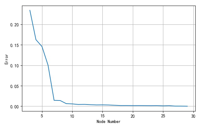
▲ 不同网络隐层节点个数对应网络训练误差
可以看到其中当网络节点大于8之后,网络训练误差就变得非常小了。
(6) 隐层节点的方差对于函数逼近的影响
为了展示RBF隐层节点的方差参数对于网络设计的影响,下面去网络隐层节点的方法从0.001变化的4的过程中,对应网络训练误差的影响。
在下面的例子中,选取隐层节点的个数
N
h
=
8
N_h = 8
Nh=8。
▲ 不同隐层节点方差对应的网络训练结果
下面显示了网络训练误差随着隐层节点方差的变化的情况。可以看出当方差在
σ
=
8
N
h
=
8
8
=
1
sigma = {8 over {N_h }} = {8 over 8} = 1
σ=Nh8=88=1附近是,对应的网络训练方差接近最小。
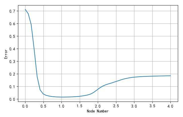
▲ 不同隐层节点方差对应网络训练误差曲线
➤※ 作业1-4中的程序
1.BP网络函数逼近程序
#!/usr/local/bin/python
# -*- coding: gbk -*-
#============================================================
# HW14BP.PY                    -- by Dr. ZhuoQing 2020-11-17
#
# Note:
#============================================================

from headm import *

#------------------------------------------------------------
# Samples data construction

random.seed(int(time.time()))

#------------------------------------------------------------
def Hermit(x):
    return 1.1 * (1 - x + 2 * x * x) * exp(-x**2/2)

x_data = random.uniform(-4, 4, 100)
y_data = Hermit(x_data) + random.normal(0, 0.1, len(x_data))

x_data = x_data.reshape(-1, 1)
y_data = y_data.reshape(1, -1)

xx = linspace(-4, 4, 250)
yy = Hermit(xx)

#------------------------------------------------------------
def shuffledata(X, Y):
    id = list(range(X.shape[0]))
    random.shuffle(id)
    return X[id], (Y.T[id]).T

#------------------------------------------------------------
# Define and initialization NN
def initialize_parameters(n_x, n_h, n_y):
    W1 = random.randn(n_h, n_x) * 0.5          # dot(W1,X.T)
    W2 = random.randn(n_y, n_h) * 0.5          # dot(W2,Z1)
    b1 = zeros((n_h, 1))                       # Column vector
    b2 = zeros((n_y, 1))                       # Column vector

    parameters = {'W1':W1,
                  'b1':b1,
                  'W2':W2,
                  'b2':b2}

    return parameters

#------------------------------------------------------------
# Forward propagattion
# X:row->sample;
# Z2:col->sample
def forward_propagate(X, parameters):
    W1 = parameters['W1']
    b1 = parameters['b1']
    W2 = parameters['W2']
    b2 = parameters['b2']

    Z1 = dot(W1, X.T) + b1                    # X:row-->sample; Z1:col-->sample
    A1 = 1/(1+exp(-Z1))
#    A1 = (1-exp(-Z1))/(1+exp(-Z1))

    Z2 = dot(W2, A1) + b2                     # Z2:col-->sample
    A2 = Z2                                   # Linear output

    cache = {'Z1':Z1,
             'A1':A1,
             'Z2':Z2,
             'A2':A2}
    return Z2, cache

#------------------------------------------------------------
# Calculate the cost
# A2,Y: col->sample
def calculate_cost(A2, Y, parameters):
    err = [x1-x2 for x1,x2 in zip(A2.T, Y.T)]
    cost = [dot(e,e) for e in err]
    return mean(cost)

#------------------------------------------------------------
# Backward propagattion
def backward_propagate(parameters, cache, X, Y):
    m = X.shape[0]                  # Number of the samples

    W1 = parameters['W1']
    W2 = parameters['W2']
    A1 = cache['A1']
    A2 = cache['A2']

    dZ2 = (A2 - Y)
    dW2 = dot(dZ2, A1.T) / m
    db2 = sum(dZ2, axis=1, keepdims=True) / m

    dZ1 = dot(W2.T, dZ2) * (A1 * (1-A1))
#    dZ1 = dot(W2.T, dZ2) * (1-A1**2)
    dW1 = dot(dZ1, X) / m
    db1 = sum(dZ1, axis=1, keepdims=True) / m

    grads = {'dW1':dW1,
             'db1':db1,
             'dW2':dW2,
             'db2':db2}

    return grads

#------------------------------------------------------------
# Update the parameters
def update_parameters(parameters, grads, learning_rate):
    W1 = parameters['W1']
    b1 = parameters['b1']
    W2 = parameters['W2']
    b2 = parameters['b2']

    dW1 = grads['dW1']
    db1 = grads['db1']
    dW2 = grads['dW2']
    db2 = grads['db2']

    W1 = W1 - learning_rate * dW1
    W2 = W2 - learning_rate * dW2
    b1 = b1 - learning_rate * db1
    b2 = b2 - learning_rate * db2

    parameters = {'W1':W1,
                  'b1':b1,
                  'W2':W2,
                  'b2':b2}

    return parameters

#------------------------------------------------------------
# Define the training
DISP_STEP           = 100

#------------------------------------------------------------
pltgif = PlotGIF()

#------------------------------------------------------------
def train(X, Y, num_iterations, learning_rate, print_cost=False):
    n_x = 1
    n_y = 1
    n_h = 10

    lr = learning_rate

    parameters = initialize_parameters(n_x, n_h, n_y)
    XX,YY = shuffledata(X, Y)

    costdim = []

    x = linspace(-4, 4, 250).reshape(-1,1)

    for i in range(0, num_iterations):
        A2, cache = forward_propagate(XX, parameters)
        cost = calculate_cost(A2, YY, parameters)
        grads = backward_propagate(parameters, cache, XX, YY)
        parameters = update_parameters(parameters, grads, lr)

        if print_cost and i % DISP_STEP == 0:
            printf('Cost after iteration:%i: %f'%(i, cost))
            costdim.append(cost)

            plt.clf()
            y,cache = forward_propagate(x, parameters)
            plt.plot(x.reshape(-1,1), y.reshape(-1,1), linewidth=3, color='r', label='Step:%d'%i)

            plt.plot(xx, yy, color='gray')
            plt.scatter(XX, YY, color='gray')
            plt.xlabel("x")
            plt.ylabel("f(x)")
            plt.grid(True)
            plt.tight_layout()
            plt.legend(loc='upper right')
            plt.draw()
            plt.pause(.1)
            pltgif.append(plt)

            if cost < 0.0001:
                break

            XX,YY = shuffledata(X, Y)

    return parameters, costdim

#------------------------------------------------------------
parameter,costdim = train(x_data, y_data, 10000, 0.5, True)
pltgif.save(r'd:temp1.gif')

printf('cost:%f'%costdim[-1])

#------------------------------------------------------------
plt.clf()
plt.plot(arange(len(costdim))*DISP_STEP, costdim)
plt.xlabel("Step(10)")
plt.ylabel("Cost")
plt.grid(True)
plt.tight_layout()
plt.show()

#------------------------------------------------------------
#        END OF FILE : HW14BP.PY
#============================================================
2.RBF网络实现程序
#!/usr/local/bin/python
# -*- coding: gbk -*-
#============================================================
# HM14RBF.PY                   -- by Dr. ZhuoQing 2020-11-19
#
# Note:
#============================================================

from headm import *

#------------------------------------------------------------
random.seed(3)

#------------------------------------------------------------
def Hermit(x):
    return 1.1 * (1 - x + 2 * x * x) * exp(-x**2/2)

x_line = linspace(-4, 4, 250)
y_line = Hermit(x_line)

RBF_SAMPLE_NUMBER       = 30
x_train = linspace(-4, 4, RBF_SAMPLE_NUMBER)
y_train = Hermit(x_train) + random.normal(0, 0.1, len(x_train))

'''
plt.plot(x_line, y_line)
plt.scatter(x_train, y_train, color='r')
plt.xlabel("x,")
plt.ylabel("f(x)")
plt.title('Hermit Function and Training Set')
plt.grid(True)
plt.tight_layout()
plt.show()
'''
#------------------------------------------------------------
# calculate the rbf hide layer output
# x: Input vector:
# H: Hide node : row->sample
# sigma: variance of RBF

def rbf_hide_out(x, H, sigma):
    Hx = H - x
    Hxx = [exp(-dot(e,e)/(sigma**2*2)) for e in Hx]
    return Hxx

def rbf(x, H, sigma, W):
    Hx = H - x
    Hxx = array([exp(-dot(e,e)/(sigma**2*2)) for e in Hx]).reshape(-1, 1)

    return (dot(W.T, Hxx))

#------------------------------------------------------------
y_train = y_train.reshape(1, -1)

def rbf_train_sim(node=10,sigma=1):
    RBF_HIDE_NODE       = node
    RBF_HIDE_SIGMA      = sigma

    Hnode = linspace(-4, 4, RBF_HIDE_NODE).reshape(-1,1) # row-->sample
    Hout = array([rbf_hide_out(x, Hnode, RBF_HIDE_SIGMA) for x in x_train]).T

    W = dot(y_train, dot(linalg.inv(eye(RBF_SAMPLE_NUMBER)*0.0001+dot(Hout.T,Hout)),Hout.T)).T

    yout = dot(W.T, Hout)
    err = yout - y_train
    error = var(err)

    return W, Hnode, error

#------------------------------------------------------------
err_dim = []
node_dim = []
pltgif = PlotGIF()

for s in linspace(0.001, 4, 50):
    W, Hnode, error = rbf_train_sim(8, s)
    err_dim.append(error)
    node_dim.append(s)

    y_rbf = [rbf(x, Hnode, s, W)[0] for x in x_line]

    plt.clf()
    plt.plot(x_line, y_line, linewidth=1, color='gray', label='origin')
    plt.scatter(x_train, y_train, color='r', label='Training data')
    plt.plot(x_line, y_rbf, linewidth=3, color='blue', label='RBF')
    plt.xlabel("x")
    plt.ylabel("f(x)")
    plt.grid(True)
    plt.title('RBF Hide Node Sigma:%5.2f'%s)
    plt.legend(loc="upper right")
    plt.tight_layout()
#    plt.show()
    plt.draw()
    plt.pause(0.1)

    pltgif.append(plt)

#------------------------------------------------------------

pltgif.save(r'd:temp1.gif')
plt.clf()
plt.plot(node_dim, err_dim)
plt.xlabel("Node Number")
plt.ylabel("Error")
plt.grid(True)
plt.tight_layout()
plt.show()

#------------------------------------------------------------
#        END OF FILE : HM14RBF.PY
#============================================================
最后
以上就是大意咖啡豆最近收集整理的关于2020人工神经网络第一次作业-参考答案第四部分➤04 第四题参考答案➤※ 作业1-4中的程序的全部内容,更多相关2020人工神经网络第一次作业-参考答案第四部分➤04内容请搜索靠谱客的其他文章。


发表评论 取消回复