【深度之眼】Pytorch框架班第五期-Week1任务3第一节：autograd与逻辑回归torch.autograd逻辑回归

78 阅读 0 评论 52 点赞

我是靠谱客的博主感动鼠标，这篇文章主要介绍【深度之眼】Pytorch框架班第五期-Week1任务3第一节：autograd与逻辑回归torch.autograd逻辑回归，现在分享给大家，希望可以做个参考。

torch.autograd

autograd-自动求导系统

torch.autograd.backward(tensors, grad_tensors=None, retain_graph=None, create_graph=False)

功能：自动求取梯度

tensors: 用于求导的张量，如loss
retain_graph: 保存计算图
create_graph: 创建导数计算图，用于高阶求导
grad_tensors: 多梯度权重

retain_graph

复制代码

1
2
3
4
5
6
7
8
9
10
11
12
13
14
15
16
17
18
19
20
21
import torch
import matplotlib.pyplot as plt
torch.manual_seed(10)



w = torch.tensor([1.], requires_grad=True)
x = torch.tensor([2.], requires_grad=True)

a = torch.add(w, x)
b = torch.add(w, 1)
y = torch.mul(a, b)

y.backward()

# y.backward()

#RuntimeError: Trying to backward through the graph a second time, but the buffers have already been freed. Specify retain_graph=True when calling backward the first time.

#y.backward(retain_graph=True)

grad_tensors

复制代码

1
2
3
4
5
6
7
8
9
10
11
12
13
14
15
16
17
18
19
20
import torch
torch.manual_seed(10)

w = torch.tensor([1.], requires_grad=True)
x = torch.tensor([2.], requires_grad=True)

a = torch.add(w, x)
b = torch.add(w, 1)

y0 = torch.mul(a, b) #dy0/dw = 5
y1 = torch.add(a, b) #dy1/dw = 2

loss = torch.cat([y0, y1], dim=0) #[y0, y1]

grad_tensors = torch.tensor([1., 2.])
loss.backward(gradient=grad_tensors)

print(w.grad)
#tensor([9.])

torch.autograd.grad(outputs, inputs, grad_inputs=None, retain_graph=None, create_graph=False)

功能：求取梯度

outputs：用于求导的张量，如loss， y
inputs: 需要梯度的张量, w
create_graph: 创建导数计算图，用于高阶求导
retain_graph: 保存计算图
grad_outputs: 多梯度权重

复制代码

1
2
3
4
5
6
7
8
9
10
11
12
13
14
15
16
17
18
19
import torch
torch.manual_seed(10)


x = torch.tensor([3.], requires_grad=True)



y = torch.pow(x, 2)   # y = x **2


grad_1 = torch.autograd.grad(y, x, create_graph=True) #grad_1 = dy/dx = 2x = 2*3 = 6
print(grad_1) # grad_1是元组  梯度 = grad_1[0]
#(tensor([6.], grad_fn=<MulBackward0>),)

grad_2 = torch.autograd.grad(grad_1[0], x) #grad_2 = d(dy/dx)/dx = d(2x)/dx = 2
print(grad_2)
# (tensor([2.]),)

autograd小贴士

1、梯度不自动清零

复制代码

1
2
3
4
5
6
7
8
9
10
11
12
13
14
15
16
17
18
19
20
21
22
23
24
25
26
import torch
torch.manual_seed(10)

w = torch.tensor([1.], requires_grad=True)
x = torch.tensor([2.], requires_grad=True)

for i in range(4):
    a = torch.add(w, x)
    b = torch.add(w, 1)
    y = torch.mul(a, b)

    y.backward()
    print(w.grad)

    #tensor([5.])
    #tensor([10.])
    #tensor([15.])
    #tensor([20.])

    w.grad.zero_()

    # tensor([5.])
    # tensor([5.])
    # tensor([5.])
    # tensor([5.])

2、依赖于叶子结点的结点，requires_grad默认为True

复制代码

1
2
3
4
5
6
7
8
9
10
11
12
13
14
import torch
torch.manual_seed(10)

w = torch.tensor([1.], requires_grad=True)
x = torch.tensor([2.], requires_grad=True)


a = torch.add(w, x)
b = torch.add(w, 1)
y = torch.mul(a, b)

print(a.requires_grad, b.requires_grad, y.requires_grad)
#True True True

3、叶子节点不执行in_place（在原始内存中改变该数据）, 如 add_， +=

复制代码

1
2
3
4
5
6
7
8
9
10
11
12
13
14
15
import torch
torch.manual_seed(10)

w = torch.tensor([1.], requires_grad=True)
x = torch.tensor([2.], requires_grad=True)


a = torch.add(w, x)
b = torch.add(w, 1)
y = torch.mul(a, b)
w.add_(1)

y.backward()
# RuntimeError: a leaf Variable that requires grad has been used in an in-place operation.

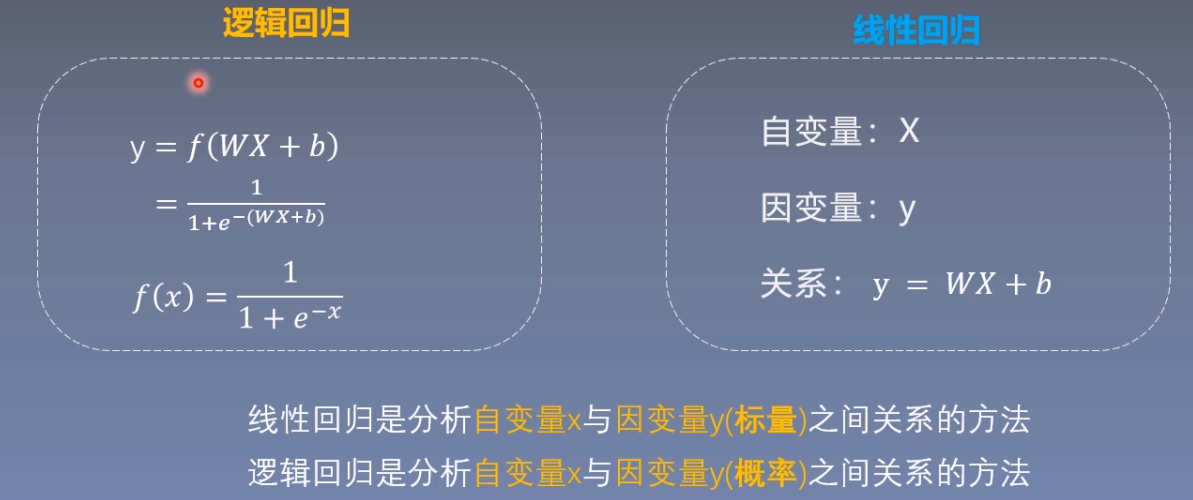
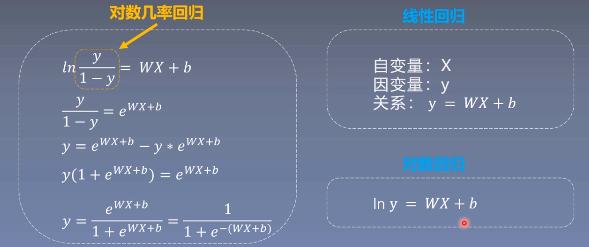
逻辑回归

逻辑回归是线性的二分类模型
模型表达式：
在这里插入图片描述

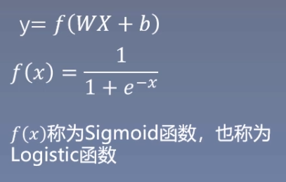
作业1：逻辑回归模型为什么可以进行二分类：

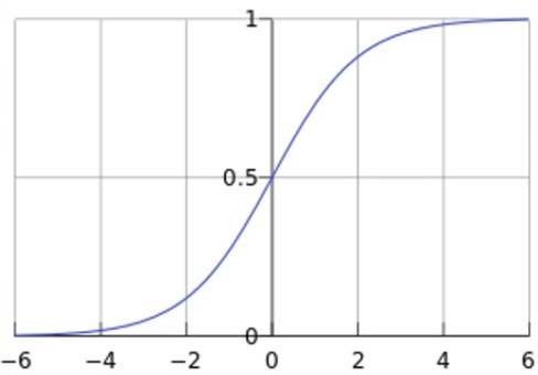
逻辑回归模型的表达式为因变量 y 等于自变量 x 的线性组合 WX+b再输入到 f(x) = 1/(1+1e-x)函数（即sigmoid函数，也称为Logistic函数）中，sigmoid函数将输入的数据映射到0~1之间，而0~1为概率取值区间，所以逻辑回归模型可以进行二分类。
在这里插入图片描述

二元逻辑回归模型的训练过程

机器学习模型训练步骤

在这里插入图片描述
步骤1：数据
步骤2：模型
步骤3：损失函数
步骤4：优化器
步骤5：迭代训练

复制代码

import torch
import torch.nn as nn
import matplotlib.pyplot as plt
import numpy as np
torch.manual_seed(10)

# ===================================== step 1/5 生成数据 =====================================
sample_nums = 100
mean_value = 1.7
bias = 1
n_data = torch.ones(sample_nums, 2)
x0 = torch.normal(mean_value * n_data, 1) + bias
y0 = torch.zeros(sample_nums)
x1 = torch.normal(-mean_value * n_data, 1) + bias
y1 = torch.ones(sample_nums)
train_x = torch.cat((x0, x1), 0)
train_y = torch.cat((y0, y1), 0)

# ===================================== step 2/5 选择模型 =====================================
class LR(nn.Module):
    def __init__(self):
        super(LR, self).__init__()
        self.features = nn.Linear(2, 1)
        self.sigmoid = nn.Sigmoid()

def forward(self, x):
        x = self.features(x)
        x = self.sigmoid(x)
        return x

lr_net = LR()  #实例化逻辑回归模型

# ===================================== step 3/5 选择损失函数 =====================================
loss_fn = nn.BCELoss()

# ===================================== step 4/5 选择优化器 =====================================
lr = 0.01 # 学习率
optimizer = torch.optim.SGD(lr_net.parameters(), lr=lr, momentum=0.9)

# ===================================== step 5/5 模型训练 =====================================
for iteration in range(1000):

#前向传播
    y_pred = lr_net(train_x)

#计算loss
    loss = loss_fn(y_pred.squeeze(), train_y)

#反向传播
    loss.backward()

#更新参数
    optimizer.step()

#绘图
    if iteration % 990 == 0:
        mask = y_pred.ge(0.5).float().squeeze() # 以0.5为阈值进行分类
        correct = (mask == train_y).sum() # 正确预测的样本个数
        acc = correct.item() / train_y.size(0) # 计算分类准确率

plt.scatter(x0.data.numpy()[:, 0], x0.data.numpy()[:, 1], c='r', label='class 0')
        plt.scatter(x1.data.numpy()[:, 0], x1.data.numpy()[:, 1], c='b', label='class 1')

w0, w1 = lr_net.features.weight[0]
        w0, w1 = float(w0.item()), float(w1.item())
        plot_b = float(lr_net.features.bias[0].item())
        plot_x = np.arange(-6, 6, 0.1)
        plot_y = (-w0 * plot_x - plot_b) / w1

plt.xlim(-5, 7)
        plt.ylim(-7, 7)
        plt.plot(plot_x, plot_y)

plt.text(-5, 5, "Loss=%.4f" % loss.data.numpy(), fontdict={'size':20, 'color': 'red'})
        plt.title("Iteration: {}nw0:{:.2f} w1:{:.2f} b: {:.2f} accuracy:{:.2%}".format(iteration, w0, w1, plot_b, acc))
        plt.legend()

plt.show()
        plt.pause(0.5)

if acc > 0.99:
            break

1
2
3
4
5
6
7
8
9
10
11
12
13
14
15
16
17
18
19
20
21
22
23
24
25
26
27
28
29
30
31
32
33
34
35
36
37
38
39
40
41
42
43
44
45
46
47
48
49
50
51
52
53
54
55
56
57
58
59
60
61
62
63
64
65
66
67
68
69
70
71
72
73
74
75
76
77
78
79
80
81
82
83
84
85
86
87
88
import torch
import torch.nn as nn
import matplotlib.pyplot as plt
import numpy as np
torch.manual_seed(10)

# ===================================== step 1/5 生成数据 =====================================
sample_nums = 100
mean_value = 1.7
bias = 1
n_data = torch.ones(sample_nums, 2)
x0 = torch.normal(mean_value * n_data, 1) + bias
y0 = torch.zeros(sample_nums)
x1 = torch.normal(-mean_value * n_data, 1) + bias
y1 = torch.ones(sample_nums)
train_x = torch.cat((x0, x1), 0)
train_y = torch.cat((y0, y1), 0)


# ===================================== step 2/5 选择模型 =====================================
class LR(nn.Module):
    def __init__(self):
        super(LR, self).__init__()
        self.features = nn.Linear(2, 1)
        self.sigmoid = nn.Sigmoid()

    def forward(self, x):
        x = self.features(x)
        x = self.sigmoid(x)
        return x

lr_net = LR()  #实例化逻辑回归模型


# ===================================== step 3/5 选择损失函数 =====================================
loss_fn = nn.BCELoss()


# ===================================== step 4/5 选择优化器 =====================================
lr = 0.01 # 学习率
optimizer = torch.optim.SGD(lr_net.parameters(), lr=lr, momentum=0.9)


# ===================================== step 5/5 模型训练 =====================================
for iteration in range(1000):

    #前向传播
    y_pred = lr_net(train_x)

    #计算loss
    loss = loss_fn(y_pred.squeeze(), train_y)

    #反向传播
    loss.backward()

    #更新参数
    optimizer.step()

    #绘图
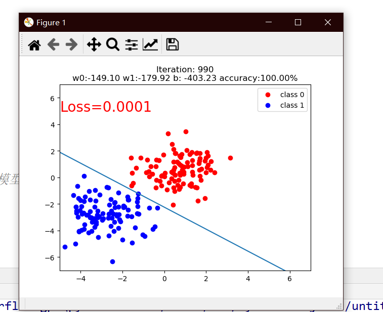
    if iteration % 990 == 0:
        mask = y_pred.ge(0.5).float().squeeze() # 以0.5为阈值进行分类
        correct = (mask == train_y).sum() # 正确预测的样本个数
        acc = correct.item() / train_y.size(0) # 计算分类准确率

        plt.scatter(x0.data.numpy()[:, 0], x0.data.numpy()[:, 1], c='r', label='class 0')
        plt.scatter(x1.data.numpy()[:, 0], x1.data.numpy()[:, 1], c='b', label='class 1')

        w0, w1 = lr_net.features.weight[0]
        w0, w1 = float(w0.item()), float(w1.item())
        plot_b = float(lr_net.features.bias[0].item())
        plot_x = np.arange(-6, 6, 0.1)
        plot_y = (-w0 * plot_x - plot_b) / w1

        plt.xlim(-5, 7)
        plt.ylim(-7, 7)
        plt.plot(plot_x, plot_y)

        plt.text(-5, 5, "Loss=%.4f" % loss.data.numpy(), fontdict={'size':20, 'color': 'red'})
        plt.title("Iteration: {}nw0:{:.2f} w1:{:.2f} b: {:.2f} accuracy:{:.2%}".format(iteration, w0, w1, plot_b, acc))
        plt.legend()

        plt.show()
        plt.pause(0.5)

        if acc > 0.99:
            break

作业2

采用代码实现逻辑回归模型的训练，并尝试调整数据生成中的mean_value，将mean_value设置为更小的值，例如1，或者更大的值，例如5，会出现什么情况？
再尝试仅调整bias，将bias调为更大或者负数，模型训练过程是怎么样的？调整mean_value,bias分别截取所训练的逻辑回归模型
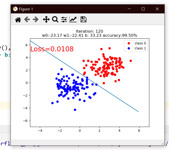
mean_value=1.7, bias=1
在这里插入图片描述
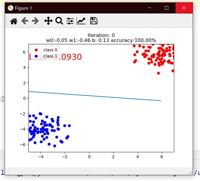
mean=1,bias=1

mean=5,bias=1

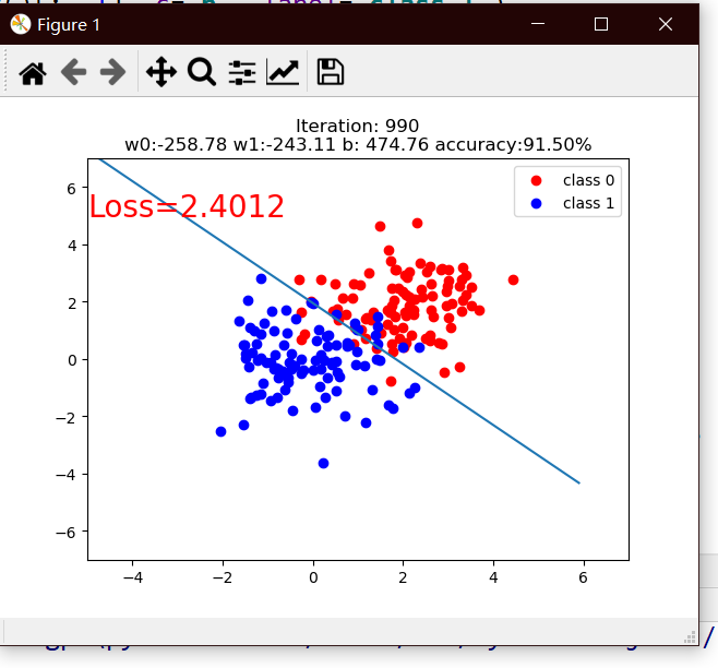
mean=1.7, bias=5

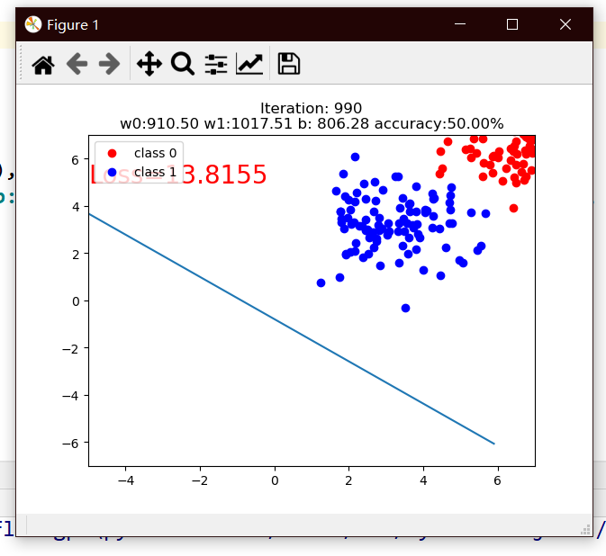
mean=1.7, bias=-1