基础知识

• 顶点（有穷）和边
  vertices and edges
• V个顶点的图最多有V（V-1）/2个边，根据数目可以判断出这个图是dense or spars.
• For an edge e that connects vertices v and w
• • v and w are adjacent (neighbours)
• • e is incident on both v and w
• Degree of a vertex 就是有几条边连入这个v。

Path

一串顶点的序列，
a sequence of vertices where each vertex has an edge to its predecessor

Simple path

A path that repeats no vertex, except that the first and last may be the same vertex.
一个没有重复顶点的路径，除了第一个和最后一个可能是同一个顶点。

Cycle

a path that is simple except last vertex = first vertex

Connected graph

there is a path from each vertex to every other vertex
if a graph is not connected, it has ≥2 connected components
一个节点到其余任何一个节点都有一个路径

Complete graph Kv

there is an edge from each vertex to every other vertex
in a complete graph, E = V(V-1)/2
每个节点 和 其他任何节点都有路径

Tree

connected (sub)graph with no cycles

Spanning tree

tree containing all vertices

• A spanning tree of connected graph G = (V,E)
• • is a subgraph of G containing all of V
• • and is a single tree (connected, no cycles)

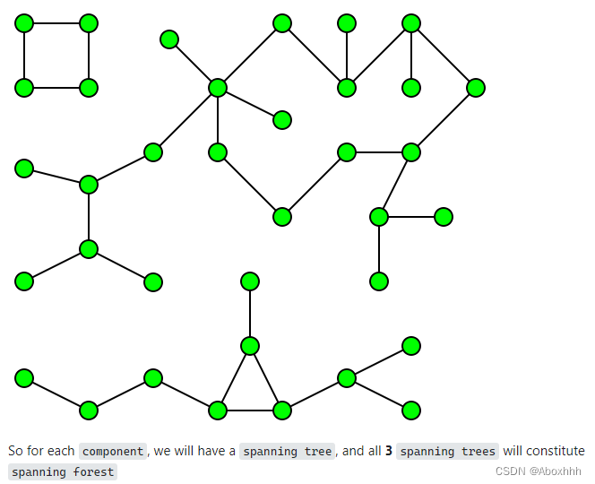
Spanning forest

• A spanning forest of non-connected graph G = (V,E) is a subgraph of G containing all of V
• • and is a set of trees (not connected, no cycles), with one tree for each connected component
    

Clique

complete subgraph

Undirected graph

edge(u,v) = edge(v,u), no self-loops (i.e. no edge(v,v))

Directed graph

edge(u,v) ≠ edge(v,u), can have self-loops (i.e. edge(v,v))

Weighted graph

each edge has an associated value (weight)
e.g. road map (weights on edges are distances between cities)

Multi-graph

allow multiple edges between two vertices
e.g. f() calls g() in several places

三种表示图的数据结构

Array of edges

通过一对顶点表示一条边。

• 添加删除边稍显复杂；
• 节省空间的表示
• 可以表示有方向的图和无方向的
  插入和删除边

1
2
3
4
5
6
insertEdge(g,(v,w)):
|  Input graph g, edge (v,w)  // assumption: (v,w) not in g
|
|  g.edges[g.nE]=(v,w)
|  g.nE=g.nE+1

1
2
3
4
5
6
7
8
9
10
removeEdge(g,(v,w)):
|  Input graph g, edge (v,w)  // assumption: (v,w) in g
|
|  i=0
|  while (v,w)≠g.edges[i] do
|     i=i+1
|  end while
|  g.edges[i]=g.edges[g.nE-1] // replace (v,w) by last edge in array
|  g.nE=g.nE-1

1
2
3
4
5
6
7
8
show(g):
|  Input graph g
|
|  for all i=0 to g.nE-1 do
|     print g.edges[i]
|  end for  
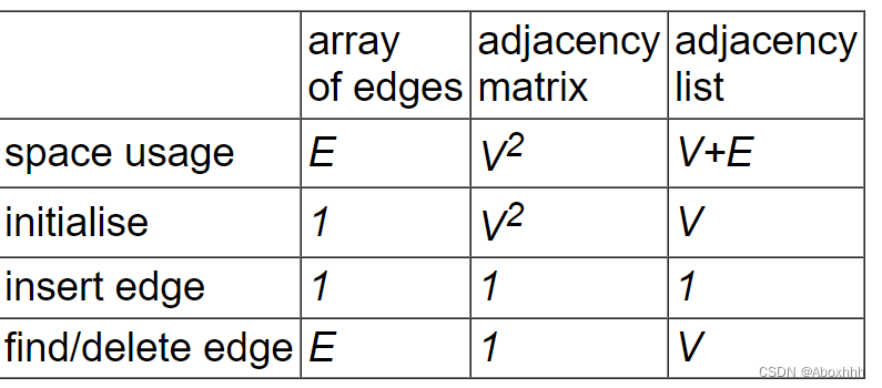
O(E)

Storage cost: O(E)
Cost of operations:

initialisation: O(1)
insert edge: O(1) (assuming edge array has space)
find/delete edge: O(E) (need to find edge in edge array)
If array is full on insert
allocate space for a bigger array, copy edges across ⇒ O(E)
If we maintain edges in order
use binary search to insert/find edge ⇒ O(log E)

Adjacency matrix

二维数组表示一条边
Advantages：

• can represent graphs, digraphs and weighted graphs
• • graphs: symmetric boolean matrix
• • digraphs: non-symmetric boolean matrix
• • weighted: non-symmetric matrix of weight values
    Disadvantages:
    if few edges (sparse) ⇒ memory-inefficient

1
2
3
4
5
6
7
8
9
10
11
12
13
Graph initialisation
newGraph(V):
|  Input  number of nodes V
|  Output new empty graph
|
|  g.nV = V   // #vertices (numbered 0..V-1)
|  g.nE = 0   // #edges
|  allocate memory for g.edges[][]
|  for all i,j=0..V-1 do
|     g.edges[i][j]=0   // false
|  end for
|  return g

1
2
3
4
5
6
7
8
9
10
Edge insertion
insertEdge(g,(v,w)):
|  Input graph g, edge (v,w)
|
|  if g.edges[v][w]=0 then  // (v,w) not in graph
|     g.edges[v][w]=1       // set to true
|     g.edges[w][v]=1
|     g.nE=g.nE+1
|  end if

1
2
3
4
5
6
7
8
9
10
Edge removal
removeEdge(g,(v,w)):
|  Input graph g, edge (v,w)
|
|  if g.edges[v][w]≠0 then  // (v,w) in graph
|     g.edges[v][w]=0       // set to false
|     g.edges[w][v]=0
|     g.nE=g.nE-1
|  end if

1
2
3
4
5
6
7
8
9
10
11
12
show(g):
|  Input graph g
|
|  for all i=0 to g.nV-2 do
|  |  for all j=i+1 to g.nV-1 do
|  |     if g.edges[i][j] then
|  |        print i"—"j
|  |     end if
|  |  end for
|  end for
Time complexity: O(V2)

Storage cost: O(V²)
If the graph is sparse, most storage is wasted.

Cost of operations:

initialisation: O(V²) (initialise V×V matrix)
insert edge: O(1) (set two cells in matrix)
delete edge: O(1) (unset two cells in matrix)

Adjacency list

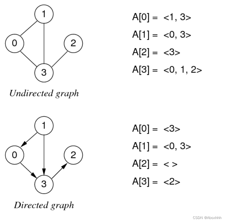
For each vertex, store linked list of adjacent vertices:

• Advantages
  relatively easy to implement in languages like C
  can represent graphs and digraphs
  memory efficient if E:V relatively small(为啥)
• Disadvantages:
  one graph has many possible representations
  (unless lists are ordered by same criterion e.g. ascending)

1
2
3
4
5
6
7
8
9
10
11
12
13
Graph initialisation
newGraph(V):
|  Input  number of nodes V
|  Output new empty graph
|
|  g.nV = V   // #vertices (numbered 0..V-1)
|  g.nE = 0   // #edges
|  allocate memory for g.edges[]
|  for all i=0..V-1 do
|     g.edges[i]=NULL   // empty list
|  end for
|  return g

1
2
3
4
5
6
7
8
Edge insertion:
insertEdge(g,(v,w)):
|  Input graph g, edge (v,w)
|
|  insertLL(g.edges[v],w)
|  insertLL(g.edges[w],v)
|  g.nE=g.nE+1

1
2
3
4
5
6
7
8
Edge removal:
removeEdge(g,(v,w)):
|  Input graph g, edge (v,w)
|
|  deleteLL(g.edges[v],w)
|  deleteLL(g.edges[w],v)
|  g.nE=g.nE-1

Storage cost: O(V+E) (V list pointers, total of 2·E list elements)
the larger of V,E determines the complexity
Cost of operations

initialisation: O(V) (initialise V lists)
insert edge: O(1) (insert one vertex into list)
if you don’t check for duplicates
find/delete edge: O(V) (need to find vertex in list)
If vertex lists are sorted
insert requires search of list ⇒ O(V)
delete always requires a search, regardless of list order

三种方法的内存空间

• array of edges ：边的数目 * 8 (即为8E)如果求最大边就是E=V*(V-1)/2
• adjacency matrix：将矩阵中的数值看作bool型，则总体大小为，指针大小乘定点个数加指针平方的个数 8*V+V²
• adjacency list: 每个节点就是顶点+内容+指针->4+4+8=16 ，每个顶点出现两次，所以总体大小就是2* 16 * E=32E，再加上前面的头指针，8*V+32E。

最后

以上就是动人耳机最近收集整理的关于20221005 数据结构之图基础知识的全部内容，更多相关20221005内容请搜索靠谱客的其他文章。