将时间序列转成图像——小波变换方法 Matlab实现1 方法2 Matlab代码实现3 结果

878 阅读 0 评论 580 点赞

我是靠谱客的博主碧蓝野狼，最近开发中收集的这篇文章主要介绍将时间序列转成图像——小波变换方法 Matlab实现1 方法2 Matlab代码实现3 结果，觉得挺不错的，现在分享给大家，希望可以做个参考。

概述

1 方法

2 Matlab代码实现

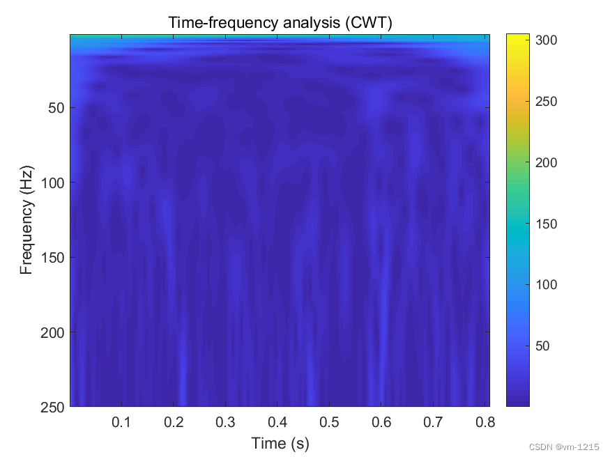
3 结果

【若觉文章质量良好且有用，请别忘了点赞收藏加关注，这将是我继续分享的动力，万分感谢！】

其他：

1.时间序列转二维图像方法及其应用研究综述_vm-1215的博客-CSDN博客

2.将时间序列转成图像——短时傅里叶方法 Matlab实现_vm-1215的博客-CSDN博客

3.将时间序列转成图像——希尔伯特-黄变换方法 Matlab实现_vm-1215的博客-CSDN博客

1 方法

小波变换(Wavelet Transform, WT)是1984年由Morlet和Grossman提出的概念，该方法承袭了短时间窗变换的局部化思想，且克服了时间-窗口大小不变的缺陷，提供了一个窗口宽度可随频率变化而变宽变窄的时频窗，从而充分突出信号的某些特征。其基本思想是：先构造一个有限长或快速衰减的母小波，然后通过缩放和平移生成多个子小波，再叠加以匹配输入信号。将其缩放尺度和平移参数对应频率和时间参数，最终得到信号的时频图。

$W_{f}(a, b)=<f, psi_{a, b}>=frac{1}{sqrt{|a|}} int_{-infty}^{+infty} f(t) psileft(frac{t-b}{a}right) d t$

其中, $psi_{a, b}$ 为母小波函数（Morlet、Ricker 等), $a$ 为尺度給数, $b$ 为平移給数。根据小波变换的定义, 给定时变信号 $f(t)$ , 其编码步骤如下：

确定参数：信号长度 $f_{len}$ , 采样频率 $sample_{rate}$ , 母小波函数, 中心频率滑动步长 $cenfre_{step}$ ;
计算最大中心频率 $cenfre_{max}=frac{sample_{rate}}{2}$ ，设置当前中心频率 $cenfre_{now}=1$ ，初始化时频矩阵 $S$ ;
根据中心频率和小波函数，构造小波曲线，再与原信号卷积，得到当前频率的时间分布向量，更新时频矩阵；
判断当前中心频率是否大于最大中心频率，若是，输出时频矩阵 $S$ ；否则，更新当前频率 $cenfre_{now}=cenfre_{now}+cenfre_{step}$ ，然后跳回步骤2。

小波变换相较于短时傅里叶变换，具有较好的时频分辨率自适应能力，更能突出实际信号的局部特征，即高频处采用低频率分辨率和高时间分辨率，低频处采用高频率分辨率和低时间分辨率。因而，小波变换在信号处理、语音处理、图像处理等领域得到广泛应用。

2 Matlab代码实现

clear, close all

%% initialize parameters
samplerate=500; % in Hz

fstep=1;   % frequency step for wavelet

%% generate simulated signals with step changes in frequency
data = csvread('3_1_link6_28_5_30min.csv');     %  input the signal from the Excle

data = data';   % change the signal from column to row

N = length(data);   % calculate the length of the data

taxis = [1:N]/samplerate;   % time axis for whole data length

figure, 
plot(taxis,data),xlim([taxis(1) taxis(end)])
xlabel('Time (s)')

%% Time-frequency analysis (CWT, morlet wavelet)
spec = tfa_morlet(data, samplerate, 1, 250, fstep);
faxis=[1:fstep:250];
Mag=abs(spec);     % get spectrum magnitude

im = figure('color',[1 1 1]);
imagesc(taxis,faxis,Mag)   % plot spectrogram as an image
colorbar
axis([taxis(1) taxis(end) faxis(1) faxis(end)])
xlabel('Time (s)')
ylabel('Frequency (Hz)')
title('Time-frequency analysis (CWT)')

saveas(im,'CWT_1.bmp')

function TFmap = tfa_morlet(td, fs, fmin, fmax, fstep)
TFmap = [];
for fc=fmin:fstep:fmax
    MW = MorletWavelet(fc/fs);  % calculate the Morlet Wavelet by giving the central freqency
    cr = conv(td, MW, 'same');  % convolution
    
    TFmap = [TFmap; abs(cr)];
end

function MW = MorletWavelet(fc)

F_RATIO = 7;    % frequency ratio (number of cycles): fc/sigma_f, should be greater than 5
Zalpha2 = 3.3;  % value of Z_alpha/2, when alpha=0.001

sigma_f = fc/F_RATIO;
sigma_t = 1/(2*pi*sigma_f);
A = 1/sqrt(sigma_t*sqrt(pi));
max_t = ceil(Zalpha2 * sigma_t);

t = -max_t:max_t;

%MW = A * exp((-t.^2)/(2*sigma_t^2)) .* exp(2i*pi*fc*t);
v1 = 1/(-2*sigma_t^2);
v2 = 2i*pi*fc;
MW = A * exp(t.*(t.*v1+v2));