1. Why study transformation
1.1 Modeling
1.2 Viewing
2. 2D transformations

Reflection Matrix
[ x ′ y ′ ] = [ − 1 0 0 1 ] [ x y ] left[begin{array}{l}x^{prime} \ y^{prime}end{array}right]=left[begin{array}{cc}-1 & 0 \ 0 & 1end{array}right]left[begin{array}{l}x \ yend{array}right] [x′y′]=[−1001][xy]
Shear Matrix
[ x ′ y ′ ] = [ 1 a 0 1 ] [ x y ] left[begin{array}{l}x^{prime} \ y^{prime}end{array}right]=left[begin{array}{ll}1 & a \ 0 & 1end{array}right]left[begin{array}{l}x \ yend{array}right] [x′y′]=[10a1][xy]
Rotation Matrix
R θ = [ cos θ − sin θ sin θ cos θ ] mathbf{R}_{theta}=left[begin{array}{cc}cos theta & -sin theta \ sin theta & cos thetaend{array}right] Rθ=[cosθsinθ−sinθcosθ]
Linear Transforms = Matrices
x
′
=
a
x
+
b
y
x^{prime}=a x+b y
x′=ax+by
y
′
=
c
x
+
d
y
y^{prime}=c x+d y
y′=cx+dy
[ x ′ y ′ ] = [ a b c d ] [ x y ] left[begin{array}{l}x^{prime} \ y^{prime}end{array}right]=left[begin{array}{ll}a & b \ c & dend{array}right]left[begin{array}{l}x \ yend{array}right] [x′y′]=[acbd][xy]
x
′
=
M
x
mathbf{x}^{prime}=mathbf{M} mathbf{x}
x′=Mx
3. Homogeneous coordinates
Translation cannot be represented in matrix form
Solution: Homogenous Coordinates
Add a third coordinate (w-coordinate)
- 2D point = (x, y, 1)T
- 2D vector = (x, y, 0)T
( x ′ y ′ w ′ ) = ( 1 0 t x 0 1 t y 0 0 1 ) ⋅ ( x y 1 ) = ( x + t x y + t y 1 ) left(begin{array}{l}x^{prime} \ y^{prime} \ w^{prime}end{array}right)=left(begin{array}{ccc}1 & 0 & t_{x} \ 0 & 1 & t_{y} \ 0 & 0 & 1end{array}right) cdotleft(begin{array}{l}x \ y \ 1end{array}right)=left(begin{array}{c}x+t_{x} \ y+t_{y} \ 1end{array}right) ⎝⎛x′y′w′⎠⎞=⎝⎛100010txty1⎠⎞⋅⎝⎛xy1⎠⎞=⎝⎛x+txy+ty1⎠⎞
why point and vector are different?
because the translation should not change the direction of vector
Valid operation if w-coordinate of result is 1 or 0
•vector + vector = vector
•point – point = vector
•point + vector = point
•point + point = ?? (meaningless) (mid point)
3.1 Affine Transformations
Affine map = linear map + translation
(
x
′
y
′
)
=
(
a
b
c
d
)
⋅
(
x
y
)
+
(
t
x
t
y
)
left(begin{array}{l}x^{prime} \ y^{prime}end{array}right)=left(begin{array}{ll}a & b \ c & dend{array}right) cdotleft(begin{array}{l}x \ yend{array}right)+left(begin{array}{l}t_{x} \ t_{y}end{array}right)
(x′y′)=(acbd)⋅(xy)+(txty)
Using homogenous coordinates:
(
x
′
y
′
1
)
=
(
a
b
t
x
c
d
t
y
0
0
1
)
⋅
(
x
y
1
)
left(begin{array}{l}x^{prime} \ y^{prime} \ 1end{array}right)=left(begin{array}{ccc}a & b & t_{x} \ c & d & t_{y} \ 0 & 0 & 1end{array}right) cdotleft(begin{array}{l}x \ y \ 1end{array}right)
⎝⎛x′y′1⎠⎞=⎝⎛ac0bd0txty1⎠⎞⋅⎝⎛xy1⎠⎞
Inverse Transform
inverse transform = invers matrix
3.2 Composite Transform
Transform Ordering Matters
R
45
⋅
T
(
1
,
0
)
≠
T
(
1
,
0
)
⋅
R
45
R_{45} cdot T_{(1,0)} neq T_{(1,0)} cdot R_{45}
R45⋅T(1,0)=T(1,0)⋅R45
Note that matrices are applied right to left:
T
(
1
,
0
)
⋅
R
45
[
x
y
1
]
=
[
1
0
1
0
1
0
0
0
1
]
[
cos
4
5
∘
−
sin
4
5
∘
0
sin
4
5
∘
cos
4
5
∘
0
0
0
1
]
[
x
y
1
]
T_{(1,0)} cdot R_{45}left[begin{array}{l}x \ y \ 1end{array}right]=left[begin{array}{ccc}1 & 0 & 1 \ 0 & 1 & 0 \ 0 & 0 & 1end{array}right]left[begin{array}{ccc}cos 45^{circ} & -sin 45^{circ} & 0 \ sin 45^{circ} & cos 45^{circ} & 0 \ 0 & 0 & 1end{array}right]left[begin{array}{l}x \ y \ 1end{array}right]
T(1,0)⋅R45⎣⎡xy1⎦⎤=⎣⎡100010101⎦⎤⎣⎡cos45∘sin45∘0−sin45∘cos45∘0001⎦⎤⎣⎡xy1⎦⎤
Decomposing Complex Transforms
4. 3D Transforms
Use homogeneous coordinates again:
•3D point = (x, y, z, 1)T
•3D vector = (x, y, z, 0)T
Use 4×4 matrices for affine transformations
(
x
′
y
′
z
′
1
)
=
(
a
b
c
t
x
d
e
f
t
y
g
h
i
t
z
0
0
0
1
)
⋅
(
x
y
z
1
)
left(begin{array}{l}x^{prime} \ y^{prime} \ z^{prime} \ 1end{array}right)=left(begin{array}{cccc}a & b & c & t_{x} \ d & e & f & t_{y} \ g & h & i & t_{z} \ 0 & 0 & 0 & 1end{array}right) cdotleft(begin{array}{l}x \ y \ z \ 1end{array}right)
⎝⎜⎜⎛x′y′z′1⎠⎟⎟⎞=⎝⎜⎜⎛adg0beh0cfi0txtytz1⎠⎟⎟⎞⋅⎝⎜⎜⎛xyz1⎠⎟⎟⎞
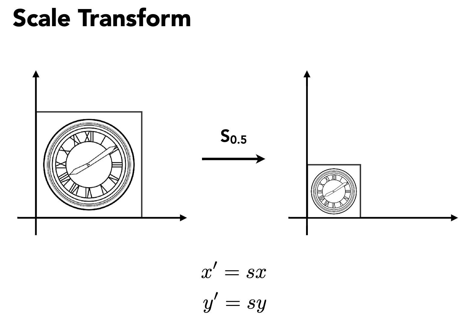
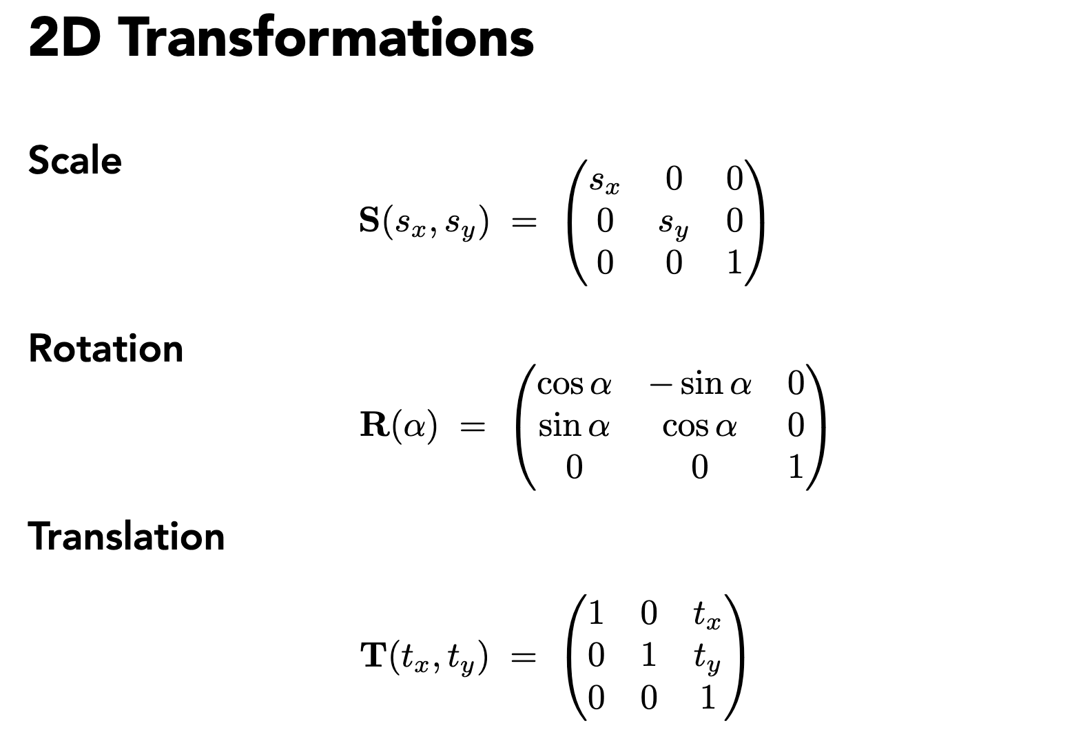
Scale
S
(
s
x
,
s
y
,
s
z
)
=
(
s
x
0
0
0
0
s
y
0
0
0
0
s
z
0
0
0
0
1
)
mathbf{S}left(s_{x}, s_{y}, s_{z}right)=left(begin{array}{cccc}s_{x} & 0 & 0 & 0 \ 0 & s_{y} & 0 & 0 \ 0 & 0 & s_{z} & 0 \ 0 & 0 & 0 & 1end{array}right)
S(sx,sy,sz)=⎝⎜⎜⎛sx0000sy0000sz00001⎠⎟⎟⎞
Translation
T
(
t
x
,
t
y
,
t
z
)
=
(
1
0
0
t
x
0
1
0
t
y
0
0
1
t
z
0
0
0
1
)
mathbf{T}left(t_{x}, t_{y}, t_{z}right)=left(begin{array}{cccc}1 & 0 & 0 & t_{x} \ 0 & 1 & 0 & t_{y} \ 0 & 0 & 1 & t_{z} \ 0 & 0 & 0 & 1end{array}right)
T(tx,ty,tz)=⎝⎜⎜⎛100001000010txtytz1⎠⎟⎟⎞
Rotation around x-, y-, or z-axis
R
x
(
α
)
=
(
1
0
0
0
0
cos
α
−
sin
α
0
0
sin
α
cos
α
0
0
0
0
1
)
mathbf{R}_{x}(alpha)=left(begin{array}{cccc}1 & 0 & 0 & 0 \ 0 & cos alpha & -sin alpha & 0 \ 0 & sin alpha & cos alpha & 0 \ 0 & 0 & 0 & 1end{array}right)
Rx(α)=⎝⎜⎜⎛10000cosαsinα00−sinαcosα00001⎠⎟⎟⎞
R
y
(
α
)
=
(
cos
α
0
sin
α
0
0
1
0
0
−
sin
α
0
cos
α
0
0
0
0
1
)
mathbf{R}_{y}(alpha)=left(begin{array}{cccc}cos alpha & 0 & sin alpha & 0 \ 0 & 1 & 0 & 0 \ -sin alpha & 0 & cos alpha & 0 \ 0 & 0 & 0 & 1end{array}right)
Ry(α)=⎝⎜⎜⎛cosα0−sinα00100sinα0cosα00001⎠⎟⎟⎞
R
z
(
α
)
=
(
cos
α
−
sin
α
0
0
sin
α
cos
α
0
0
0
0
1
0
0
0
0
1
)
mathbf{R}_{z}(alpha)=left(begin{array}{cccc}cos alpha & -sin alpha & 0 & 0 \ sin alpha & cos alpha & 0 & 0 \ 0 & 0 & 1 & 0 \ 0 & 0 & 0 & 1end{array}right)
Rz(α)=⎝⎜⎜⎛cosαsinα00−sinαcosα0000100001⎠⎟⎟⎞
Compose any 3D rotation
R
x
y
z
(
α
,
β
,
γ
)
=
R
x
(
α
)
R
y
(
β
)
R
z
(
γ
)
mathbf{R}_{x y z}(alpha, beta, gamma)=mathbf{R}_{x}(alpha) mathbf{R}_{y}(beta) mathbf{R}_{z}(gamma)
Rxyz(α,β,γ)=Rx(α)Ry(β)Rz(γ)
So-called Euler angles; Often used in flight simulators: roll, pitch, yaw
Rotation by angle αaround axis n
R
(
n
,
α
)
=
cos
(
α
)
I
+
(
1
−
cos
(
α
)
)
n
n
T
+
sin
(
α
)
(
0
−
n
z
n
y
n
z
0
−
n
x
−
n
y
n
x
0
)
mathbf{R}(mathbf{n}, alpha)=cos (alpha) mathbf{I}+(1-cos (alpha)) mathbf{n} mathbf{n}^{T}+sin (alpha)left(begin{array}{ccc}0 & -n_{z} & n_{y} \ n_{z} & 0 & -n_{x} \ -n_{y} & n_{x} & 0end{array}right)
R(n,α)=cos(α)I+(1−cos(α))nnT+sin(α)⎝⎛0nz−ny−nz0nxny−nx0⎠⎞
一般情况下,说明沿某个轴的方向旋转,都默认该轴是经过原点的。
若是沿任意轴(不经过原点)旋转,则先平移再旋转再平移。
5. Viewing transformation
5.1 View / Camera transformation
Think about how to take a photo
-Find a good place and arrange people (model transformation)
-Find a good “angle” to put the camera (view transformation)
-Cheese! (projection transformation)
MVP变换
Define the camera first
- Position e ⃗ vec{e} e
- Look-at / gaze direction g ^ hat{g} g^
- Up direction t ^ hat{t} t^ (assuming perp. to look-at)
How about that we always transform the camera to
- The origin, up at Y, look at -Z
- And transform the objects along with the camera
Transform the camera by M v i e w M_{v i e w} Mview
So it’s located at the origin, up at Y, look at -Z
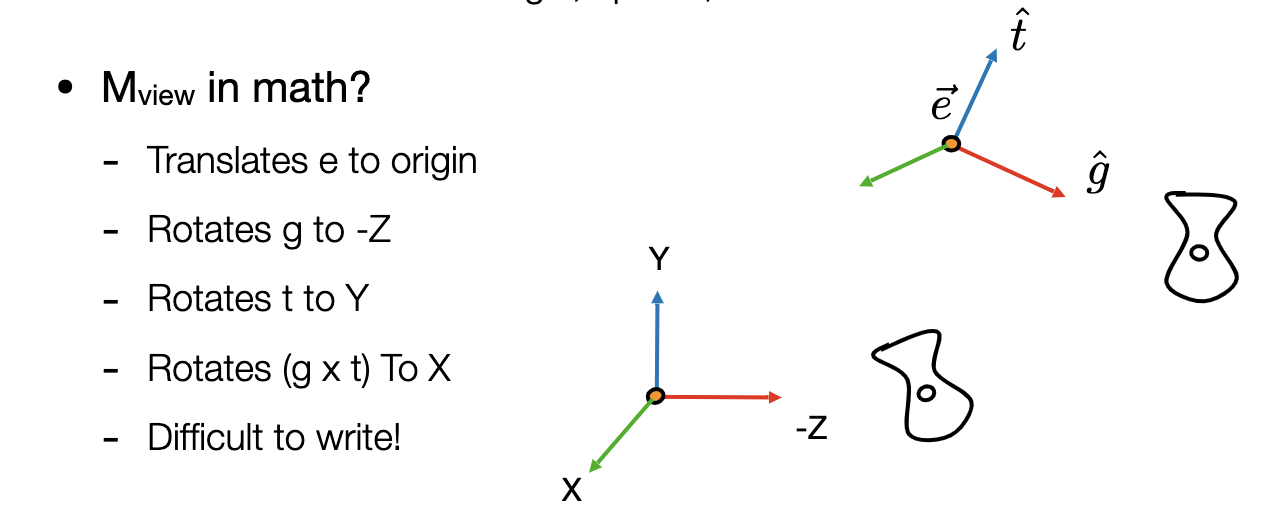
M view M_{text {view}} Mview in math
- Let’s write M view = R view T view M_{text {view}}=R_{text {view}} T_{text {view}} Mview=RviewTview
- Translate e to origin
T v i e w = [ 1 0 0 − x e 0 1 0 − y e 0 0 1 − z e 0 0 0 1 ] T_{v i e w}=left[begin{array}{cccc} 1 & 0 & 0 & -x_{e} \ 0 & 1 & 0 & -y_{e} \ 0 & 0 & 1 & -z_{e} \ 0 & 0 & 0 & 1 end{array}right] Tview=⎣⎢⎢⎡100001000010−xe−ye−ze1⎦⎥⎥⎤ - Rotate g to − z , t -z, t −z,t to Y , ( g × t ) Y,(g times t) Y,(g×t) To X X X
- Consider its inverse rotation:
X
X
X to
(
g
×
t
)
,
Y
(g times t), Y
(g×t),Y to
t
,
Z
t, Z
t,Z to
−
g
-g
−g
R v i e w − 1 = [ x g ^ × t ^ x t x − g 0 y g ^ × t ^ y t y − g 0 z g ^ × t ^ z t z − g 0 0 0 0 1 ] R_{v i e w}^{-1}=left[begin{array}{cccc}x_{hat{g} times hat{t}} & x_{t} & x_{-g} & 0 \ y_{hat{g} times hat{t}} & y_{t} & y_{-g} & 0 \ z_{hat{g} times hat{t}} & z_{t} & z_{-g} & 0 \ 0 & 0 & 0 & 1end{array}right] Rview−1=⎣⎢⎢⎡xg^×t^yg^×t^zg^×t^0xtytzt0x−gy−gz−g00001⎦⎥⎥⎤
因为旋转矩阵是正交矩阵,所以求逆=求转置。
R v i e w = [ x g ^ × t ^ y g ^ × t ^ z g ^ × t ^ 0 x t y t z t 0 x − g y − g z − g 0 0 0 0 1 ] R_{v i e w}=left[begin{array}{cccc}x_{hat{g} times hat{t}} & y_{hat{g} times hat{t}} & z_{hat{g} times hat{t}} & 0 \ x_{t} & y_{t} & z_{t} & 0 \ x_{-g} & y_{-g} & z_{-g} & 0 \ 0 & 0 & 0 & 1end{array}right] Rview=⎣⎢⎢⎡xg^×t^xtx−g0yg^×t^yty−g0zg^×t^ztz−g00001⎦⎥⎥⎤
Summary
-Transform objects together with the camera
-Until camera’s at the origin, up at Y, look at -Z
•Also known as ModelView Transformation
•But why do we need this? For projection transformation!
5.2 Projection transformation
正交投影和透视投影
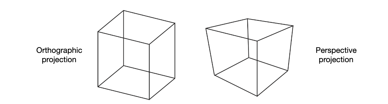
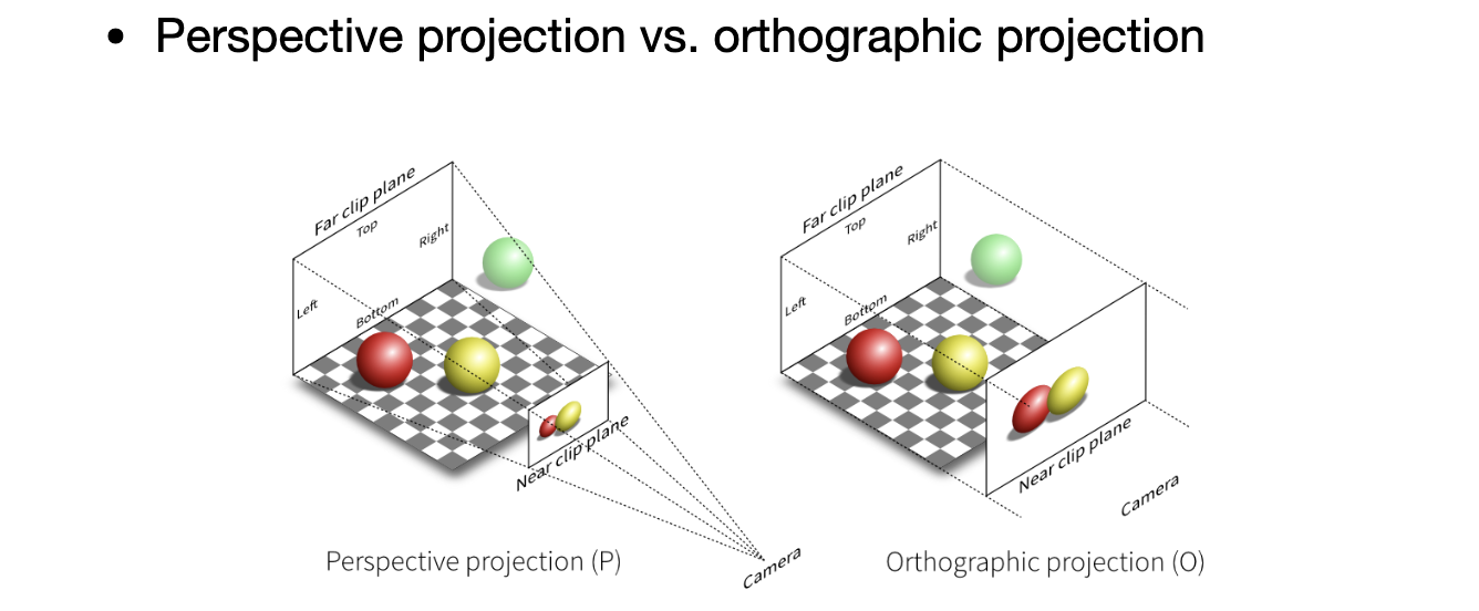
5.2.1 Orthographic projection
A simple way of understanding
- Camera located at origin, looking at - Z Z Z, up at Y Y Y (looks familiar?)
- Drop Z coordinate
- Translate and scale the resulting rectangle to
[
−
1
,
1
]
2
[-1,1]^{2}
[−1,1]2 #这样做可以方便以后的计算
存在问题:如何区分物体的前后
In general
- We want to map a cuboid [ l , r ] × [ b , t ] × [ f , n ] [l, r] times [b, t] times[f, n] [l,r]×[b,t]×[f,n] to the "canonical (正则、规范、标准)”cube [-1, 1]3
Slightly different orders (to the “simple way”)
- Center cuboid by translating
- Scale into “canonical” cube
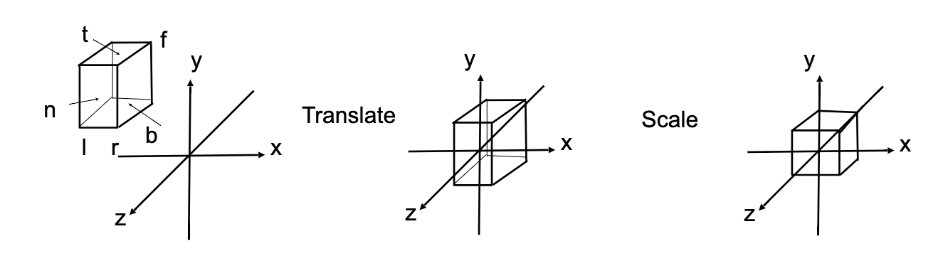
定义的立方体中,l是left,r是right,在x轴上;b是bottom,t是top,在y轴上;
f是far,n是near,在z轴上,但是这里注意z轴上是远的地方数值更小,因为是看-z方向。(然而,在一些API中,例如OpenGL中是定义的左手系,就不存在这个问题;但是这样的话x和y叉乘就不是z)
Transformation matrix
- Translate (center to origin) first, then scale (length/width/height to 2)
M ortho = [ 2 r − l 0 0 0 0 2 t − b 0 0 0 0 2 n − f 0 0 0 0 1 ] [ 1 0 0 − r + l 2 0 1 0 − t + b 2 0 0 1 − n + f 2 0 0 0 1 ] M_{text {ortho}}=left[begin{array}{cccc}frac{2}{r-l} & 0 & 0 & 0 \ 0 & frac{2}{t-b} & 0 & 0 \ 0 & 0 & frac{2}{n-f} & 0 \ 0 & 0 & 0 & 1end{array}right]left[begin{array}{cccc}1 & 0 & 0 & -frac{r+l}{2} \ 0 & 1 & 0 & -frac{t+b}{2} \ 0 & 0 & 1 & -frac{n+f}{2} \ 0 & 0 & 0 & 1end{array}right] Mortho=⎣⎢⎢⎡r−l20000t−b20000n−f200001⎦⎥⎥⎤⎣⎢⎢⎡100001000010−2r+l−2t+b−2n+f1⎦⎥⎥⎤
5.2.2 Perspective projection
•Most common in Computer Graphics, art, visual system
•Further objects are smaller
•Parallel lines not parallel; converge to single point

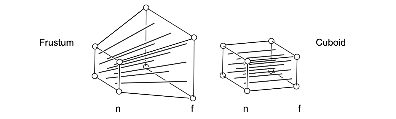
How to do perspective projection
- First “squish” the frustum into a cuboid ( n − > n , f − > f ) ( M persp->ortho ) (mathrm{n}->mathrm{n}, mathrm{f}->mathrm{f})left(mathrm{M}_{text {persp->ortho }}right) (n−>n,f−>f)(Mpersp->ortho )
- Do orthographic projection (Mortho, already known!)
In order to find a transformation
- Find the relationship between transformed points (x’, y’, z’) and the original points
(
x
,
y
,
z
)
(x, y, z)
(x,y,z)
y ′ = n z y x ′ = n z x (similar to y’) y^{prime}=frac{n}{z} y quad x^{prime}=frac{n}{z} x text { (similar to y') } y′=znyx′=znx (similar to y’)
In homogeneous coordinates,
(
x
y
z
1
)
⇒
(
n
x
/
z
n
y
/
z
unknown
1
)
mult.
(
n
x
n
y
by
z
still unknown
z
)
left(begin{array}{l} x \ y \ z \ 1 end{array}right) Rightarrowleft(begin{array}{c} n x / z \ n y / z \ text { unknown } \ 1 end{array}right) begin{array}{l} text { mult. }left(begin{array}{c} n x \ n y \ text { by } z \ text { still unknown } \ z end{array}right) end{array}
⎝⎜⎜⎛xyz1⎠⎟⎟⎞⇒⎝⎜⎜⎛nx/zny/z unknown 1⎠⎟⎟⎞ mult. ⎝⎜⎜⎜⎜⎛nxny by z still unknown z⎠⎟⎟⎟⎟⎞
So the “squish” (persp to ortho) projection does this
M
p
e
r
s
p
→
o
r
t
h
o
(
4
×
4
)
(
x
y
z
1
)
=
(
n
x
n
y
unknown
z
)
M_{p e r s p rightarrow o r t h o}^{(4 times 4)}left(begin{array}{l} x \ y \ z \ 1 end{array}right)=left(begin{array}{c} n x \ n y \ text { unknown } \ z end{array}right)
Mpersp→ortho(4×4)⎝⎜⎜⎛xyz1⎠⎟⎟⎞=⎝⎜⎜⎛nxny unknown z⎠⎟⎟⎞
Already good enough to figure out part of
M
persp->ortho
mathrm{M}_{text {persp->ortho }}
Mpersp->ortho
M
p
e
r
s
p
→
o
r
t
h
o
=
(
n
0
0
0
0
n
0
0
?
?
?
?
0
0
1
0
)
M_{p e r s p rightarrow o r t h o}=left(begin{array}{llll} n & 0 & 0 & 0 \ 0 & n & 0 & 0 \ ? & ? & ? & ? \ 0 & 0 & 1 & 0 end{array}right) quad
Mpersp→ortho=⎝⎜⎜⎛n0?00n?000?100?0⎠⎟⎟⎞
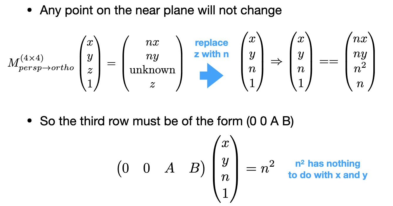
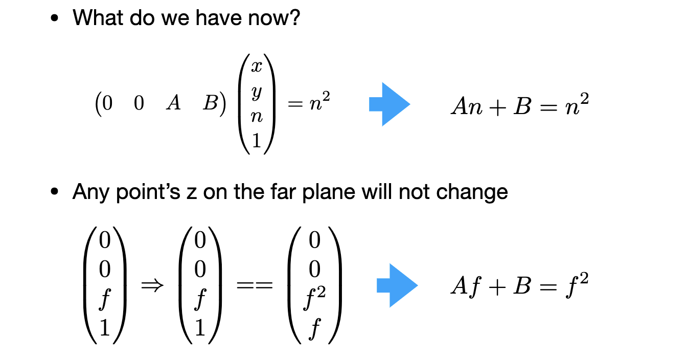
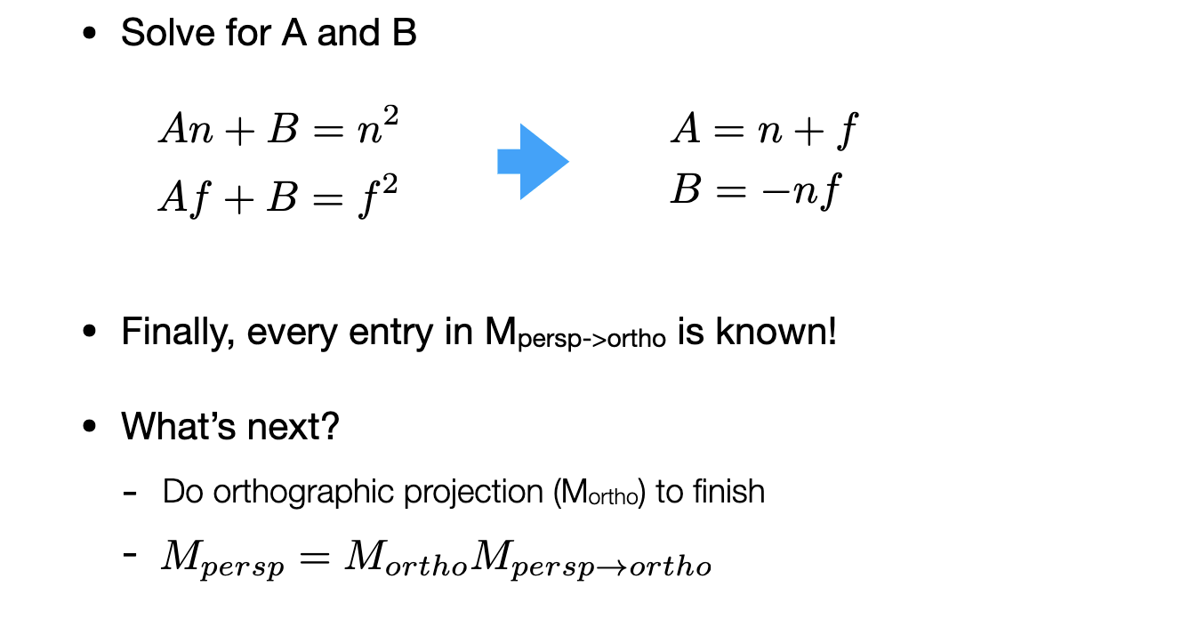
Observation: the third row is responsible for z ′ z^{prime} z′
- Any point on the near plane will not change
- Any point’s z on the far plane will not change
下面是推导和原理
最后
以上就是和谐手链最近收集整理的关于Lecture 3 Transformation1. Why study transformation2. 2D transformations3. Homogeneous coordinates4. 3D Transforms5. Viewing transformation的全部内容,更多相关Lecture内容请搜索靠谱客的其他文章。


![[leetcode] 356. Line Reflection 解题报告](https://www.shuijiaxian.com/files_image/reation/bcimg22.png)


发表评论 取消回复